R (CRAN)

Analysis: R Programming Language

1. Characterizing the Open Source Software Ecosystem

All CRAN Packages (As of September 2023)

1.1 What is the distribution of R Packages and R Package maintainers by sector?

Out of 19,852 packages, we were not able to identify a sector for 12,721 of them. For the ones where a sector was found (7131), 6240 were identified as academic, 583 as business, 166 as government, and 142 as nonprofit

Code

## sectors based on packages
pander(table(cran$Sector, useNA = "always"))

Academic	Business	Government	Nonprofit	Unknown	NA
6240	583	166	142	12721	0

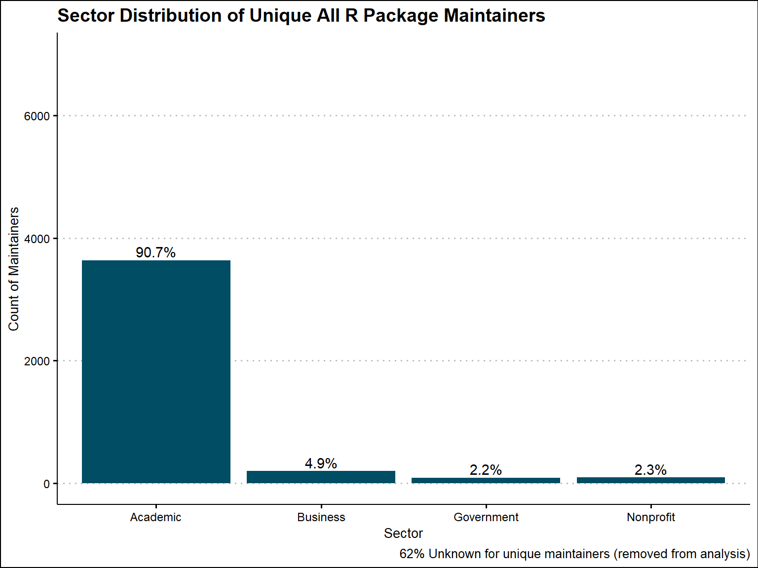
Out of 10,821 unique maintainers, we were able to identify a sector for 4,014 of them. 3,639 are from the academic sector, 196 from the business sector, 87 from the government sector, and 92 from nonprofit sector

Code

## sectors based on unique maintainers
cran_unique <- cran %>%
                    distinct(email, .keep_all = T)

pander(table(cran_unique$Sector, useNA = "always"))

Academic	Business	Government	Nonprofit	Unknown	NA
3639	196	87	92	6807	0

Based on all CRAN Packages that we were able to extract a sector from, 88% are academic, 8% are business, 2% are government, and 2% are nonprofit. When looking at the unique maintainers, 91% are academic, 5% are business, 2% are government, and 2% are nonprofit.

Code

# Calculate counts by sector (All packages)
cran_sector_counts <- cran %>%
  filter(Sector != "Unknown") %>%
  count(Sector) %>%
  mutate(proportion = n / sum(n),
         proportion_label = paste0(round(proportion * 100, 1), "%")) 

# Save plot
cran_sector_counts_plot <- ggplot(cran_sector_counts, aes(x = Sector, y = n)) +
  geom_bar(stat = "identity", fill = '#014d64') +
  geom_text(aes(label = proportion_label), vjust = -0.3) +
  ylab("Count of Packages") +
  ylim(c(0, 7000))+
  ggtitle(label = "Sector Distribution of All R packages")+
  labs(caption = "*64% Unknown for packages (removed from analysis)")+
  theme_clean()

cran_sector_counts_plot

# Calculate counts by sector (For unique Maintainers)
cran_sector_counts_unique <- cran %>%
  distinct(email, .keep_all = T)%>%
  filter(Sector != "Unknown") %>%
  count(Sector) %>%
  mutate(proportion = n / sum(n),
         proportion_label = paste0(round(proportion * 100, 1), "%")) 

# Save plot
cran_sector_counts_unique_plot <-ggplot(cran_sector_counts_unique, aes(x = Sector, y = n)) +
  geom_bar(stat = "identity", fill = '#014d64') +
  geom_text(aes(label = proportion_label), vjust = -0.3) +
  ylab("Count of Maintainers") +
  ylim(c(0, 7000))+
  ggtitle(label = "Sector Distribution of Unique All R Package Maintainers")+ 
  labs(caption = "62% Unknown for unique maintainers (removed from analysis)")+
  theme_clean()

cran_sector_counts_unique_plot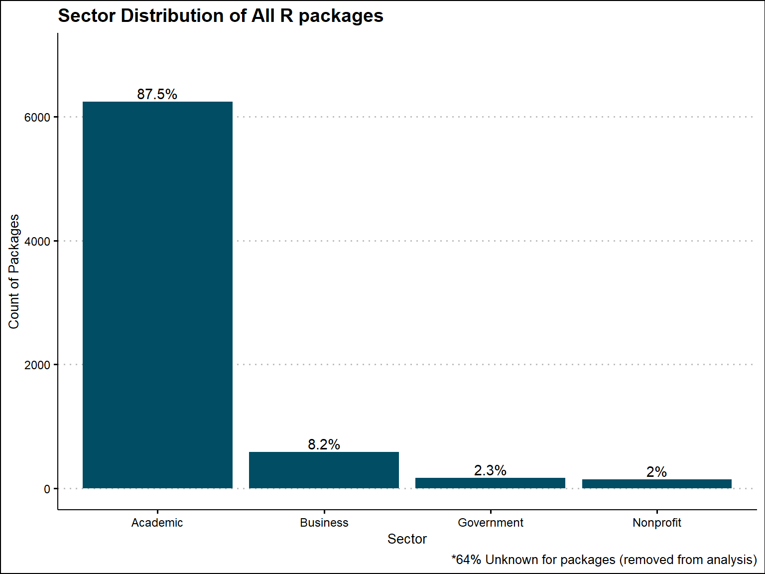

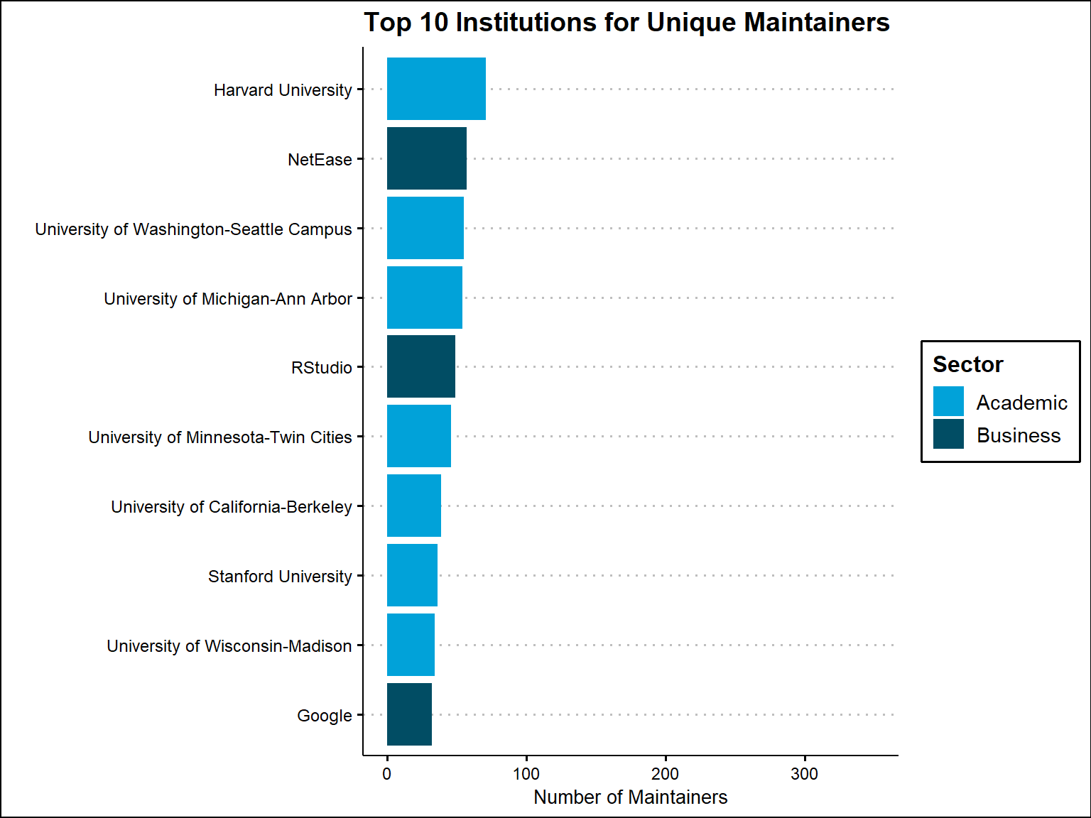
1.2 What are the top 10 institutions developing R Packages based on the number of packages and number of unique maintainers?

Based on all packages, the most frequent institution identified in the maintainer email domains is Rstudio followed by Harvard University. However, if we base it on unique maintainer email domains, then Harvard becomes most frequently identified institution, followed by Rstudio. It appears that a lot of the packages developed from Rstudio domains are the same ones.

Code

### sorting to the top 10 most common institutions for packages
top10_Institutions <- sort(table(cran$Institution), decreasing = T)
top10_Institutions <- as.data.frame(head(top10_Institutions, 10))

colnames(top10_Institutions) <- c("Institution", "Freq")

### joining to institution dataframe to get sector variable
top10_Institutions <- cran %>% 
  right_join(top10_Institutions, by = "Institution")%>%
  distinct(Institution, .keep_all = T)%>%
  select(Institution, Sector, Freq)%>%
  arrange(desc(Freq))

### sorting to the top 10 most common institutions for distinct maintainers
top10_Institutions_unique <- sort(table(cran_unique$Institution), decreasing = T)
top10_Institutions_unique <- as.data.frame(head(top10_Institutions_unique, 10))

colnames(top10_Institutions_unique) <- c("Institution", "Freq")

### joining to institution unique dataframe to get sector variable
top10_Institutions_unique <- cran %>% 
  right_join(top10_Institutions_unique, by = "Institution")%>%
  distinct(Institution, .keep_all = T)%>%
  select(Institution, Sector, Freq)%>%
  arrange(desc(Freq))

### Graph output of top 10 institutions for packages
 ggplot(top10_Institutions, aes(x = reorder(Institution, Freq), y = Freq, fill = Sector))+
   geom_bar(stat = "identity") +
    coord_flip() +
    scale_y_continuous(expand = c(0,0)) +
    labs(x = "", y = "Number of Packages",
         title = "Top 10 Institutions for All R Packages" ) +
    ylim(c(0, 350))+
  scale_fill_economist()+
  theme_clean()


 
 ### Graph output of top 10 institutions for unique maintainers
 ggplot(top10_Institutions_unique, aes(x = reorder(Institution, Freq), y = Freq, fill = Sector))+
   geom_bar(stat = "identity") +
    coord_flip() +
    scale_y_continuous(expand = c(0,0)) +
    labs(x = "", y = "Number of Maintainers",
         title = "Top 10 Institutions for Unique Maintainers" ) +
    ylim(c(0, 350))+
  scale_fill_economist()+
  theme_clean()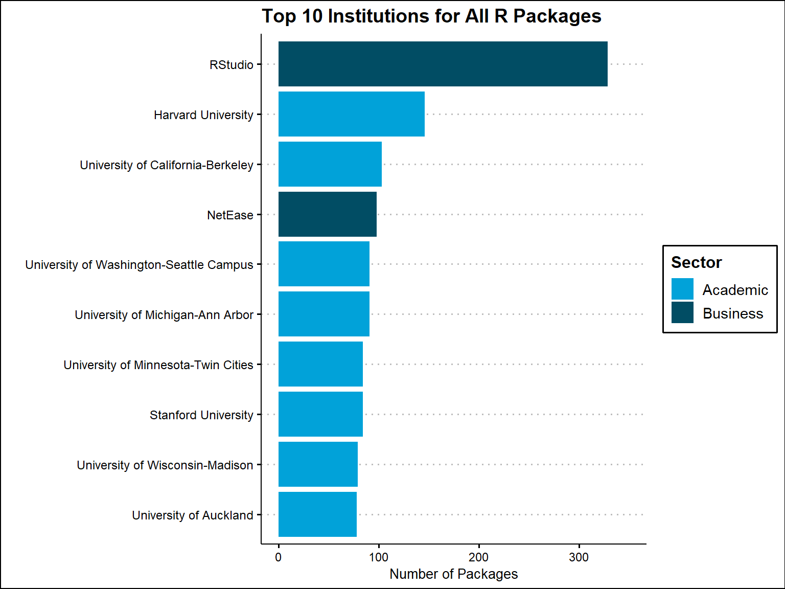

Code

### Table output of top 10 Institutions for packages
top10_Institutions %>%
  kbl(caption = "Most Frequent Institutions for Packages", escape = F)%>%
  kable_classic()%>%
  kable_styling(font_size = 12,  full_width = T)%>%
 row_spec(0, bold = T, background = '#014d64', color = "white")%>%
  column_spec(1:2, border_right = T)%>%
  scroll_box()

Most Frequent Institutions for Packages

Institution	Sector	Freq
RStudio	Business	329
Harvard University	Academic	146
University of California-Berkeley	Academic	103
NetEase	Business	98
University of Washington-Seattle Campus	Academic	91
University of Michigan-Ann Arbor	Academic	91
University of Minnesota-Twin Cities	Academic	84
Stanford University	Academic	84
University of Wisconsin-Madison	Academic	79
University of Auckland	Academic	78

Code

### Table output of top 10 Institutions for unique maintainers
top10_Institutions_unique %>%
  kbl(caption = "Most Frequent Institutions for Unique Maintainers", escape = F)%>%
  kable_classic()%>%
  kable_styling(font_size = 12,  full_width = T)%>%
 row_spec(0, bold = T, background = '#014d64', color = "white")%>%
  column_spec(1:2, border_right = T)%>%
  scroll_box()

Most Frequent Institutions for Unique Maintainers

Institution	Sector	Freq
Harvard University	Academic	71
NetEase	Business	57
University of Washington-Seattle Campus	Academic	55
University of Michigan-Ann Arbor	Academic	54
RStudio	Business	49
University of Minnesota-Twin Cities	Academic	46
University of California-Berkeley	Academic	39
Stanford University	Academic	36
University of Wisconsin-Madison	Academic	34
Google	Business	32

2. GitHub R Packages

As stated in the introduction, we also collected data from GitHub for all R packages that we were able to identify with a repository. Github provides us with more data including repository statistics and data at the contributor level, which would be each individual that is a collaborator on a given repository. We can now look at distributions at both the maintainer and contributor levels to compare. For now, we’ll still just be looking at the package level, meaning the maintainer level information of the packages.

After linking to GitHub, we are able to identify repository data for 7,844 out of the 19,852 packages on CRAN

We first have to extract the slug from all packages that have a GitHub URL

Code

#### filtering for URLs that only contain github.com in the link
cran_github <- cran %>% filter(grepl("https://github.com", URL, ignore.case = TRUE))

### extracting the URL portion with the slug
cran_github <- cran_github %>%
          mutate(URL = str_extract(URL, "https://github.com/([^/]+)/([^/]+)"))


### removing commas
cran_github <- cran_github %>%
          mutate(URL = sub(",.*$",  "",  URL))

### extracting slug portion
cran_github <- cran_github %>%
          mutate(slug = str_extract(URL, "(?<=github.com/)[^/]+/[^/]+"))


cran_github <- cran_github %>%
          mutate(slug = str_extract(slug, "[^\\s]+/[^\\s]+"))

We can now join the original cran dataframe to the repositories we collected data for

Code

### Read in package repository data
cran_repos <- dbReadTable(con, "package_repo_info")
### creating slug for linkage
cran_repos <- cran_repos %>%
  mutate(slug = paste(owner, repo, sep = "/"))

### join to cran by Package for more data
cran_repos <- cran_github %>%
                  left_join(cran_repos, by = "slug")%>%
                  distinct(slug, .keep_all = T)


### create "year_created" variable
cran_repos$year_created <- substr(cran_repos$created_at, 1, 4)

2.1 What is the distribution of GitHub R Packages and GitHub R Package maintainers by sector?

Out of 7,844 packages identified on GitHub, we were able to identify a sector for 2379 of them. For the ones where a sector was found, 1858 were identified as academic, 385 as business, 70 as government, and 66 as nonprofit

Code

pander(table(cran_repos$Sector, useNA = "always"))

Academic	Business	Government	Nonprofit	Unknown	NA
1858	385	70	66	5465	0

Out of 4267 unique maintainers identified on GitHub, we were able to identify a sector for 1322 of them. 1132 were identified as academic, 109 as business, 39 as government, and 42 as nonprofit

Code

## sectors based on unique maintainers
cran_repos_unique <- cran_repos %>%
                    distinct(email, .keep_all = T)

pander(table(cran_repos_unique$Sector, useNA = "always"))

Academic	Business	Government	Nonprofit	Unknown	NA
1132	109	39	42	2945	0

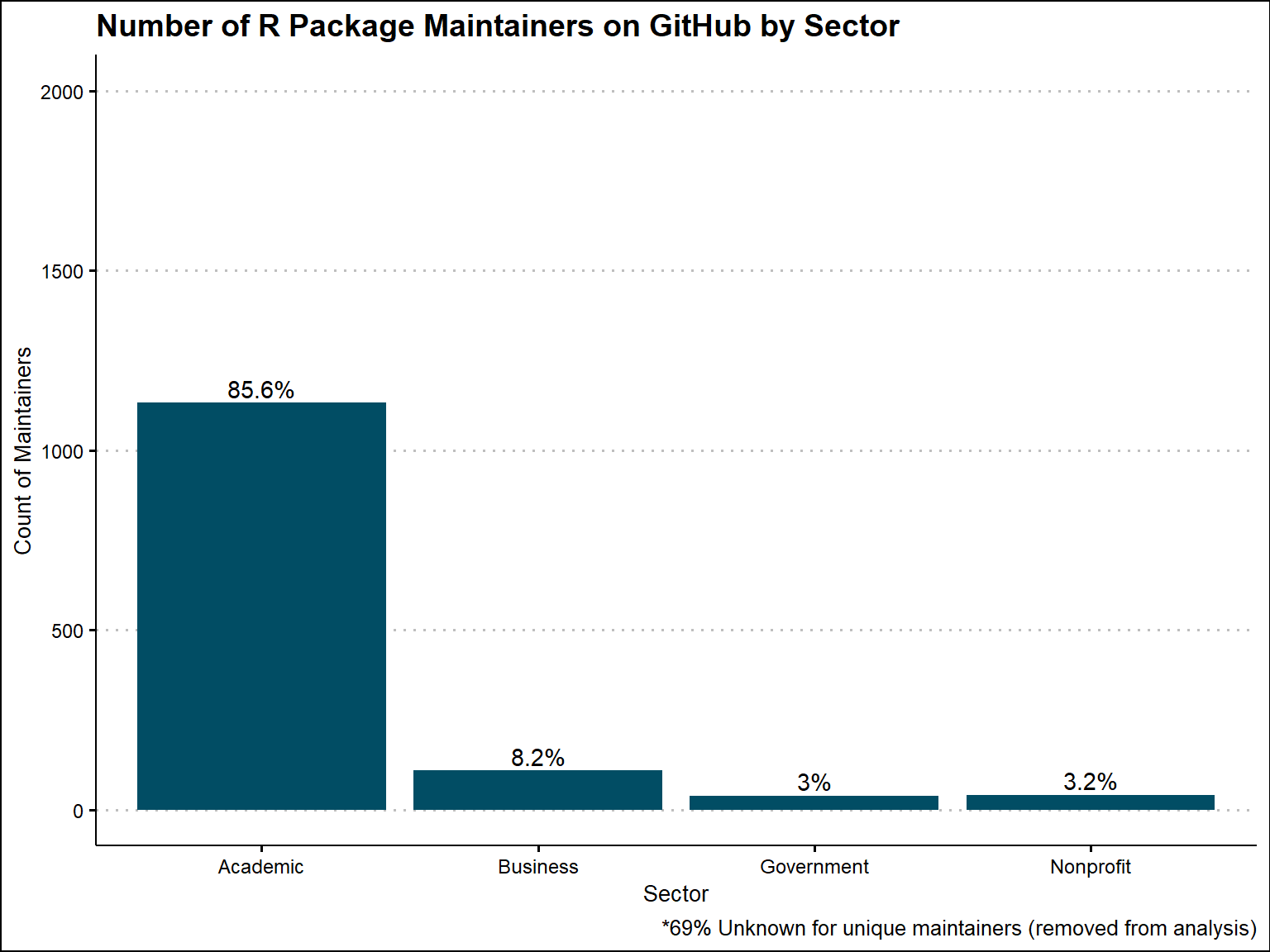
Based on all GitHub R Packages that we were able to extract a sector from, 78% are academic, 16% are business, 3% are government, and 3% are nonprfoit. When looking at the unique maintainers, 86% are academic, 8% are business, 3% are government, and 3% are nonprofit.

Code

# Calculate counts by sector (All packages on GitHub)
cran_repo_sector_counts <- cran_repos %>%
  filter(Sector != "Unknown") %>%
  count(Sector) %>%
  mutate(proportion = n / sum(n),
         proportion_label = paste0(round(proportion * 100, 1), "%")) 

# Save plot
cran_repo_sector_counts_plot <- ggplot(cran_repo_sector_counts, aes(x = Sector, y = n)) +
  geom_bar(stat = "identity", fill = '#014d64') +
  geom_text(aes(label = proportion_label), vjust = -0.3) +
  ylab("Count of Packages") +
  ylim(c(0, 2000))+
  ggtitle(label = "Number of R Packages on GitHub by Maintainer's Sector")+ 
  labs(caption = "*70% Unknown for packages (removed from analysis)")+
  theme_clean()

cran_repo_sector_counts_plot

# Calculate counts by sector (For unique Maintainers on GitHub)
cran_repo_sector_counts_unique <- cran_repos_unique %>%
  distinct(email, .keep_all = T)%>%
  filter(Sector != "Unknown") %>%
  count(Sector) %>%
  mutate(proportion = n / sum(n),
         proportion_label = paste0(round(proportion * 100, 1), "%")) 

# Save plot
cran_repo_sector_counts_unique_plot <-ggplot(cran_repo_sector_counts_unique, aes(x = Sector, y = n)) +
  geom_bar(stat = "identity", fill = '#014d64') +
  geom_text(aes(label = proportion_label), vjust = -0.3) +
  ylab("Count of Maintainers") +
  ylim(c(0, 2000))+
  ggtitle(label = "Number of R Package Maintainers on GitHub by Sector")+
  labs(caption = "*69% Unknown for unique maintainers (removed from analysis)")+
  theme_clean()

cran_repo_sector_counts_unique_plot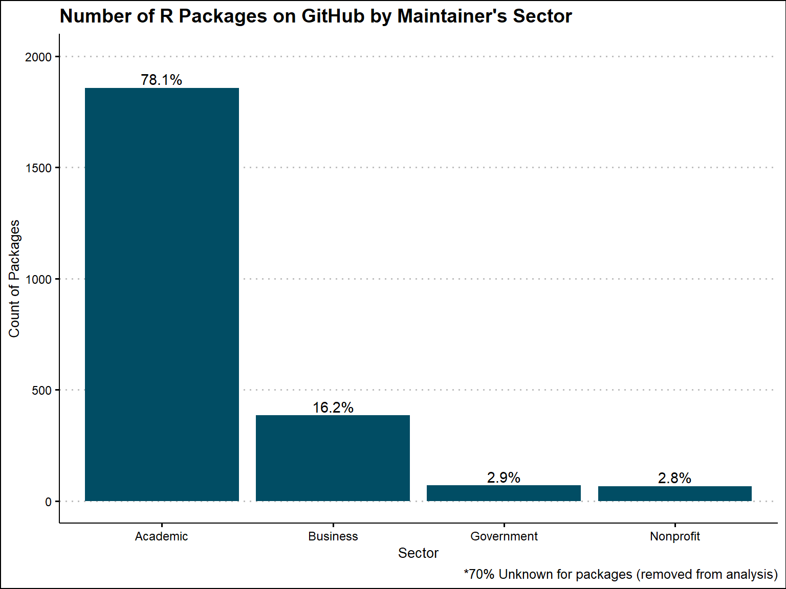

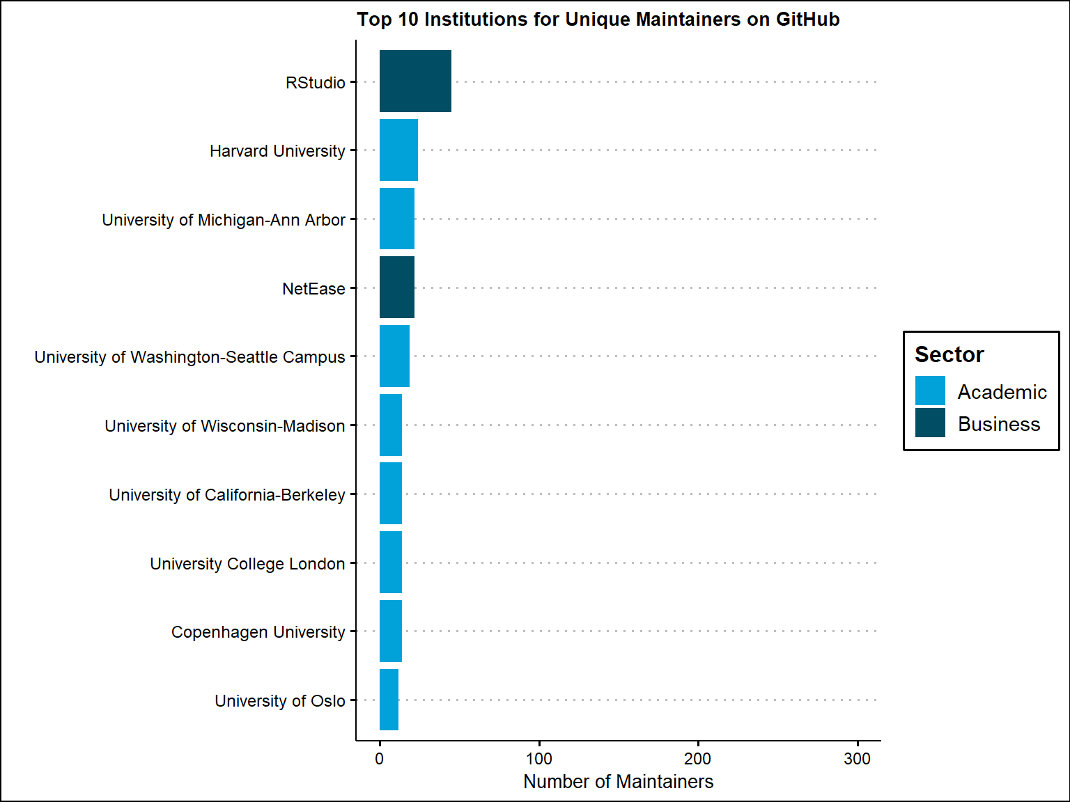
2.2 What are the top 10 institutions developing R Packages on GitHub based on the number of packages and number of unique maintainers?

For number of packages overall, Rstudio develops the most R packages on Github by a good margin. However, if we look at the unique maintainers only, the spread between Rstudio and other institutions becomes much smaller. It seems that their are a few maintainers that develop a lot of the R packages. We also note that those who do not have a sector will also not have an institution label (these coincide with one another).

Code

### sorting to the top 10 most common institutions for packages
top10_Institutions_GitHub <- sort(table(cran_repos$Institution), decreasing = T)
top10_Institutions_GitHub <- as.data.frame(head(top10_Institutions_GitHub, 10))

colnames(top10_Institutions_GitHub) <- c("Institution", "Freq")

### joining to institution dataframe to get sector variable
top10_Institutions_GitHub <- cran_repos %>% 
  right_join(top10_Institutions_GitHub, by = "Institution")%>%
  distinct(Institution, .keep_all = T)%>%
  select(Institution, Sector, Freq)%>%
  arrange(desc(Freq))

### sorting to the top 10 most common institutions for distinct maintainers
top10_Institutions_GitHub_unique <- sort(table(cran_repos_unique$Institution), decreasing = T)
top10_Institutions_GitHub_unique <- as.data.frame(head(top10_Institutions_GitHub_unique, 10))

colnames(top10_Institutions_GitHub_unique) <- c("Institution", "Freq")

### joining to institution unique dataframe to get sector variable
top10_Institutions_GitHub_unique <- cran_repos_unique %>% 
  right_join(top10_Institutions_GitHub_unique, by = "Institution")%>%
  distinct(Institution, .keep_all = T)%>%
  select(Institution, Sector, Freq)%>%
  arrange(desc(Freq))

### Graph output of top 10 institutions for packages
 ggplot(top10_Institutions_GitHub, aes(x = reorder(Institution, Freq), y = Freq, fill = Sector))+
   geom_bar(stat = "identity") +
    coord_flip() +
    scale_y_continuous(expand = c(0,0)) +
    labs(x = "", y = "Number of Packages",
         title = "Top 10 Institutions for R Packages on GitHub" ) +
    ylim(c(0, 300))+
  scale_fill_economist()+
  theme_clean()+
   theme(
  plot.title = element_text(size = 10))


 
 ### Graph output of top 10 institutions for unique maintainers
 ggplot(top10_Institutions_GitHub_unique, aes(x = reorder(Institution, Freq), y = Freq, fill = Sector))+
   geom_bar(stat = "identity") +
    coord_flip() +
    scale_y_continuous(expand = c(0,0)) +
    labs(x = "", y = "Number of Maintainers",
         title = "Top 10 Institutions for Unique Maintainers on GitHub" ) +
    ylim(c(0, 300))+
  scale_fill_economist()+
  theme_clean()+
   theme(
  plot.title = element_text(size = 10))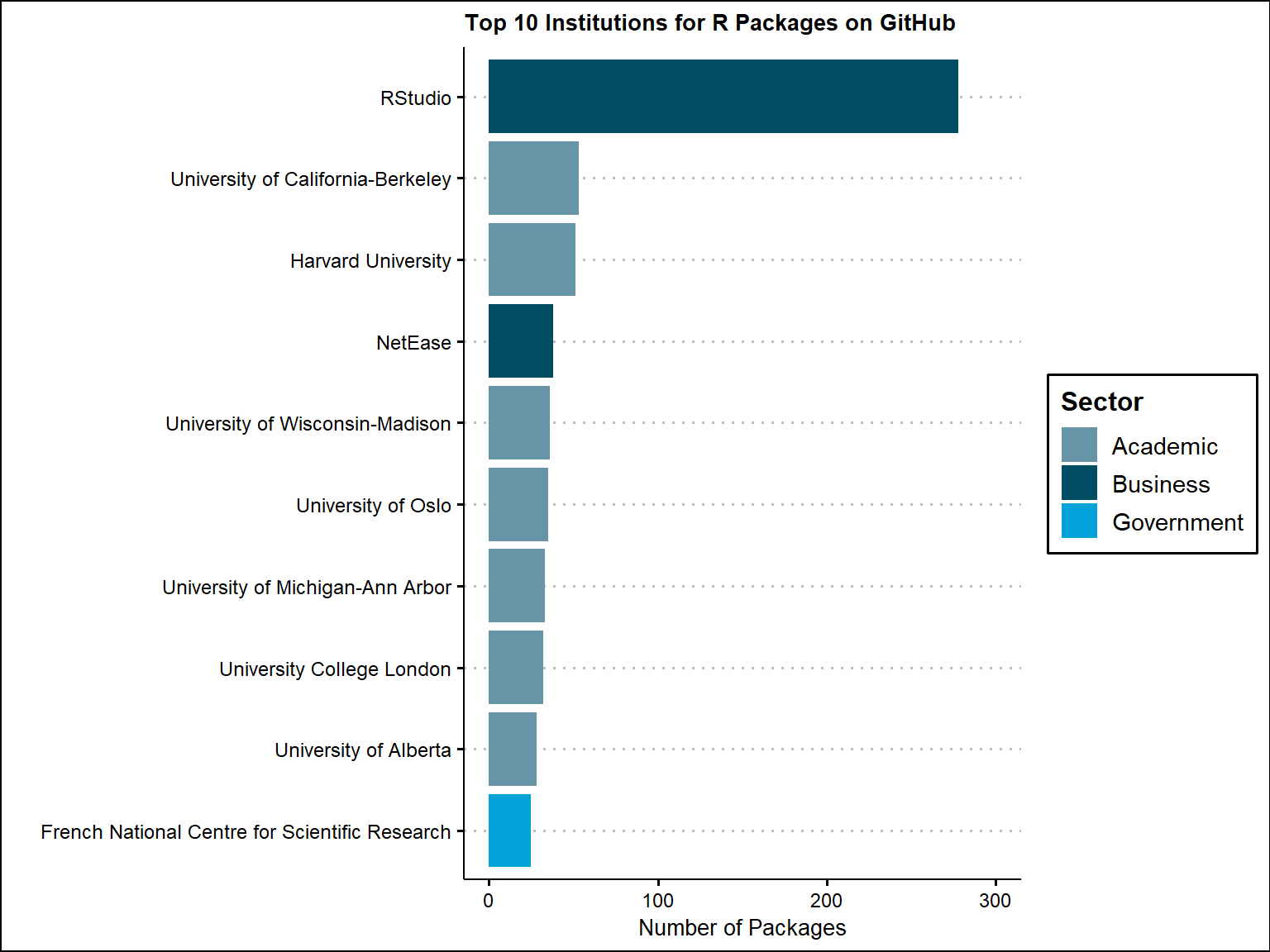

Code

### Table output of top 10 Institutions for packages
top10_Institutions_GitHub %>%
  kbl(caption = "Most Frequent Institutions for Packages on GitHub", escape = F)%>%
  kable_classic()%>%
  kable_styling(font_size = 12,  full_width = T)%>%
 row_spec(0, bold = T, background = '#014d64', color = "white")%>%
  column_spec(1:2, border_right = T)%>%
  scroll_box()

Most Frequent Institutions for Packages on GitHub

Institution	Sector	Freq
RStudio	Business	278
University of California-Berkeley	Academic	53
Harvard University	Academic	51
NetEase	Business	38
University of Wisconsin-Madison	Academic	36
University of Oslo	Academic	35
University of Michigan-Ann Arbor	Academic	33
University College London	Academic	32
University of Alberta	Academic	28
French National Centre for Scientific Research	Government	25

Code

### Table output of top 10 Institutions for unique maintainers
top10_Institutions_GitHub_unique %>%
  kbl(caption = "Most Frequent Institutions for Unique Maintainers on GitHub", escape = F)%>%
  kable_classic()%>%
  kable_styling(font_size = 12,  full_width = T)%>%
 row_spec(0, bold = T, background = '#014d64', color = "white")%>%
  column_spec(1:2, border_right = T)%>%
  scroll_box()

Most Frequent Institutions for Unique Maintainers on GitHub

Institution	Sector	Freq
RStudio	Business	45
Harvard University	Academic	24
University of Michigan-Ann Arbor	Academic	22
NetEase	Business	22
University of Washington-Seattle Campus	Academic	19
University of California-Berkeley	Academic	14
University College London	Academic	14
University of Wisconsin-Madison	Academic	14
Copenhagen University	Academic	14
University of Oslo	Academic	12

2.3 How are these distributions changing over time?

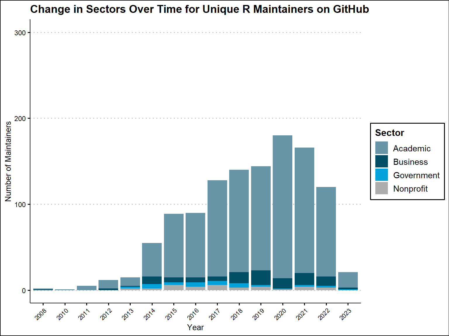
We can identify the year created by looking at the date and time the repository was created on github. This is one of the variables we collected during GitHub data collection.

We can now see how the distribution of sectors is changing over time and also identify patterns in years where we were able to identify the most sectors. We do the same type of analysis, one for sectors of all R packages on GitHub and one for sectors of all unique R maintainers on GitHub .

It looks like the ability to identify a sector generally increases from year to year all the way up until 2020, where there is a dip in the number of packages and maintainers being registered on GitHub. As for the sector distribution, it essentially stays the same from year to year for both plots. Academic makes a majority of the distribution, while there are slight fluctuations in the other sectors.

Code

cran_repos_time <- cran_repos %>%
  filter(Sector != "Unknown" & year_created != "NA" ) %>%
ggplot(aes(x = as.factor(year_created), fill = Sector)) +
  geom_bar() +
  labs(
    x = "Year",
    y = "Number of Packages",
    title = "Change in Sectors Over Time for R Packages on GitHub"
  ) +
  theme_clean()+
  scale_fill_economist()+
  theme(axis.text.x = element_text(angle = 45, hjust = 1, size = 8))+
  ylim(c(0, 300))

cran_repos_time


cran_repos_unique_time <- cran_repos_unique %>%
  filter(Sector != "Unknown" & year_created != "NA" ) %>%
ggplot(aes(x = as.factor(year_created), fill = Sector)) +
  geom_bar() +
  labs(
    x = "Year",
    y = "Number of Maintainers",
    title = "Change in Sectors Over Time for Unique R Maintainers on GitHub"
  ) +
  theme_clean()+
  scale_fill_economist()+
  theme(axis.text.x = element_text(angle = 45, hjust = 1, size = 8))+
  ylim(c(0, 300))


cran_repos_unique_time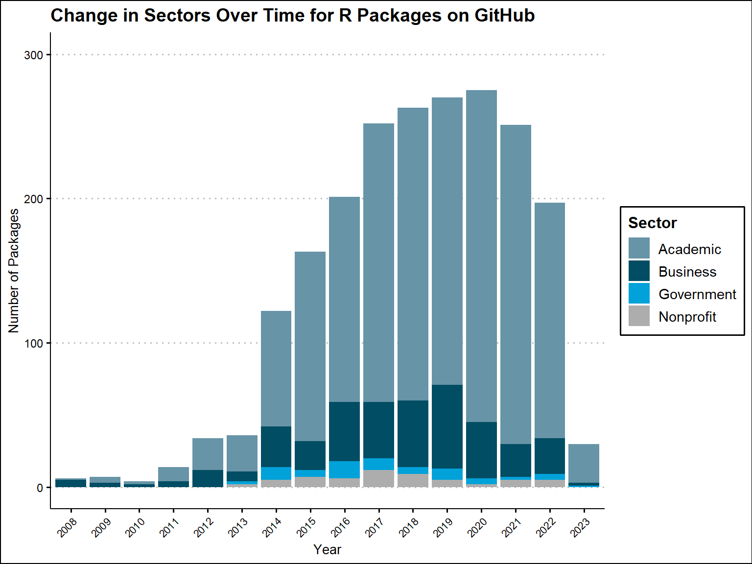

3. GitHub R Package Contributors

Now we look at distributions of all R contributors on GitHub. After GitHub data collection, we were able to identify 14328 unique R contributors.

Code

### Read in contributor data
cran_users <- dbReadTable(con, "cran_users_sectors")

cran_users_unique <- cran_users %>%
                        distinct(login, .keep_all = T)

### commits of each user
user_commits <- dbReadTable(con, "cran_gh_commits_by_login")

We also collected commit data for each of the unique R contributors. We join this back with our unique R contributors dataframe to combine commit, sector, country, and organization variables.

Code

### summing up total commits for all unique users of unique repos
user_commits_total <- user_commits %>%
                  group_by(slug, login) %>%
                  summarise(total_additions = sum(additions)) %>%
                  ungroup()

### join back to unique users dataframe for other variables
user_commits_total <- user_commits_total %>%
                        left_join(cran_users_unique, by = "login") %>%
                          select(slug, login,name, email, total_additions, organization, sector, country)

cran_repos2 <- cran_repos %>%
                select(slug, year_created, stargazer_count, fork_count, Downloads_All_Time, Downloads_Normalized)

user_commits_total <- user_commits_total %>%
                        left_join(cran_repos2, by = "slug")


### Rename NA sectors to Unknown 
user_commits_total <- user_commits_total %>%
  mutate(sector = ifelse(is.na(sector) | sector == "Unknown", "Unknown", sector))

3.1 What is the distribution of unique GitHub R contributors by sector?

For the 14,328 unique R contributors on GitHub, we were able to identify a sector for 2,573 of them. 1870 coming from academic, 482 from business, 137 from nonprofit, and 137 from nonprofit

Code

pander(table(cran_users_unique$sector, useNA = "always"))

Academic	Business	Government	Nonprofit	Unknown	NA
1870	482	84	137	11755	0

For unique R developers (contributors to a slug) on GitHub, 73% are identified as academic, 19% as business, 5% as nonprofit, and 3% as government.

Code

# Calculate counts by sector (All packages on GitHub)
cran_user_sector_counts <- cran_users_unique %>%
  filter(sector != "NA" & sector != "Unknown") %>%
  count(sector) %>%
  mutate(proportion = n / sum(n),
         proportion_label = paste0(round(proportion * 100, 1), "%")) %>%
  arrange(desc(proportion)) %>%
  mutate(sector = factor(sector, levels = unique(sector)))

# Save plot
cran_user_sector_counts_plot <- ggplot(cran_user_sector_counts, aes(x = sector, y = n)) +
  geom_bar(stat = "identity", fill = '#014d64') +
  geom_text(aes(label = proportion_label), vjust = -0.3) +
  ylab("Count of Developers") +
  ylim(c(0, 2000))+
  ggtitle(label = "Number of R Package Developers on GitHub by Sector")+ 
  labs(caption = "*Developers without sector information are removed in this figure (82% of 14,328 R Developers)")+
  theme_clean()

cran_user_sector_counts_plot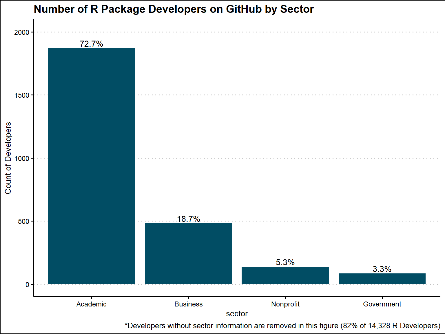

3.1.1 How do we attribute contribution to sectors (equal)?

We now aim to try to attribute contribution to sectors with a couple of methods. First, we look at equal contribution, where each member of a repository is given an equal fraction of credit regardless of level of contribution. So, if a repository has five members, each member will get .2 credit, and then the fractions are aggregated to the sectors. We will count the fraction to unknown sectors as well, but we will remove it in any graphical displays, as we already know this will be the highest percentage.

Note: This is different than looking at unique user distribution, as it will count repeat users if they are members of multiple repositories

Code

# 1. Count the number of unique login per slug.
login_counts <- user_commits_total %>%
  group_by(slug) %>%
  summarise(num_logins = n_distinct(login))

# 2. Compute the contribution fraction for each login.
user_commits_total <- user_commits_total %>%
  left_join(login_counts, by = "slug") %>%
  mutate(contribution_fraction_equal = 1 / num_logins) %>%
  select(-num_logins)  # Removing the num_logins column as it's no longer needed

# 3. Sum the contribution fraction for each sector per slug.
sector_contribution <- user_commits_total %>%
  group_by(slug, sector) %>%
  summarise(total_contribution_fraction = sum(contribution_fraction_equal))

# 4. Aggregate the contribution fraction for each sector across all slugs.
sector_aggregated <- sector_contribution %>%
  group_by(sector) %>%
  summarise(overall_contribution_fraction = sum(total_contribution_fraction))


# Calculate the total overall contribution fraction over all sectors
total_overall_contribution = sum(sector_aggregated$overall_contribution_fraction)

# Calculate the percentage contribution for each sector
sector_aggregated = sector_aggregated %>%
  mutate(percentage_contribution = round((overall_contribution_fraction / total_overall_contribution) * 100, 1))

### Plot percentage contribution
sector_aggregated$percentage_label <- scales::percent(sector_aggregated$percentage_contribution / 100)

Based on equal contribution of each unique login to each unique repository, we would attribute 80% of credit to the academic sector, 15% to the business, 2% to the government, and 3% to the nonprofit. Note that we removed Unknown from the distribution, where we would have to attribute 78% to. So, the percentage distrbutions listed here are based on the percentage we do know.

Code

### Excluding the unknown percentage in the table
total_excluding_unknown <- sum(sector_aggregated$overall_contribution_fraction[sector_aggregated$sector != "Unknown"])

### recalculating what percentages would be without unknown 
sector_aggregated <- sector_aggregated %>%
  mutate(percentage_contribution_excl_unknown = ifelse(sector != "Unknown", 
                                                       round((overall_contribution_fraction / total_excluding_unknown) * 100, 1), NA_real_))

### making labels
sector_aggregated$percentage_label_excl_unknown <- scales::percent(sector_aggregated$percentage_contribution_excl_unknown / 100, accuracy = 0.1)

ggplot(sector_aggregated %>% filter(sector != "Unknown"), aes(x = sector, y = percentage_contribution_excl_unknown)) +
  geom_bar(stat = "identity", fill = '#014d64') +
  geom_text(aes(label = percentage_label_excl_unknown), vjust = -0.5, size = 4) + # Adjust vjust and size as needed
  labs(title = "Percentage Contribution by Sector (Equal Code)",
       x = "Sector",
       y = "Percentage Contribution") +
  theme_clean() +
  labs(caption = "*Excludes the percentage contribution from unknown sector (77.7%)")+
  ylim(0,100)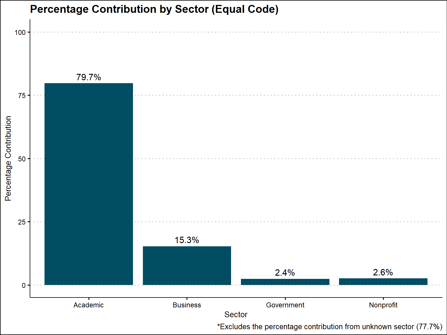

3.1.2 How do we attribute contribution to sectors (Additions based)?

We also can attribute contribution to sectors based on the lines of code written for a unique user of a given repository. The more lines of code added for that repository, the more credit that user will get. So, if a repository has 500 total lines of code, and one user wrote 300 of them, he/she would get .6 of the credit. We again apply the fractional counting method to the sectors after calculating this.

Code

# Calculate the total code additions for each slug (project/repository identifier)
# Grouping by the slug, and then summarizing the total additions for each slug.
slug_totals <- user_commits_total %>%
  group_by(slug) %>%
  summarise(total_code_for_slug = sum(total_additions))

# Compute the contribution fraction for each user.
# This is done by joining the user's total additions with the total code additions for their respective slug,
# and then computing the user's contribution as a fraction of the slug's total.
user_commits_total <- user_commits_total %>%
  left_join(slug_totals, by = "slug") %>%
  mutate(contribution_fraction_loc = total_additions / total_code_for_slug)

# Compute the total contribution fraction for each combination of slug and sector.
# This groups the data by slug and sector, and then sums up the contribution fractions.
sector_addition_contribution <- user_commits_total %>%
  group_by(slug, sector) %>%
  summarise(total_addition_contribution = sum(contribution_fraction_loc))

# Aggregate the contributions at the sector level.
# This groups by the sector and then computes the overall contribution fraction for each sector.
sector_aggregated_additions <- sector_addition_contribution %>%
  group_by(sector) %>%
  summarise(overall_addition_contribution = sum(total_addition_contribution, na.rm = TRUE))

# Compute the total overall additions across all sectors.
total_overall_additions = sum(sector_aggregated_additions$overall_addition_contribution)

# Calculate the percentage of additions for each sector relative to the total overall additions.
sector_aggregated_additions$percentage_additions = round((sector_aggregated_additions$overall_addition_contribution / total_overall_additions) * 100,1)

# Create a label for the percentage values, turning the decimal fraction into a percentage string (e.g., 0.5 becomes "50%").
sector_aggregated_additions$percentage_label_additions = scales::percent(sector_aggregated_additions$percentage_additions / 100)

After doing these calculations, we now see that 83% an be attributed to the academic sector, 13% to the business, 2% to the government, and 2% to the nonprofit. The original amount attributed to Unknown decreased to 75.6%

Code

# Calculate the total code additions while excluding the 'Unknown' sector.
total_excluding_unknown_add <- sum(sector_aggregated_additions$overall_addition_contribution[sector_aggregated_additions$sector != "Unknown"])

# Compute the percentage contribution for each sector relative to the total (excluding 'Unknown' sector).
# If the sector is 'Unknown', set the percentage as NA.
sector_aggregated_additions <- sector_aggregated_additions %>%
  mutate(percentage_contribution_excl_unknown = ifelse(sector != "Unknown", 
                                                       round((overall_addition_contribution / total_excluding_unknown_add) * 100, 1), NA_real_))

# Create a label for the percentage values that excludes 'Unknown' sector, turning the decimal fraction into a percentage string.
sector_aggregated_additions$percentage_label_excl_unknown <- scales::percent(sector_aggregated_additions$percentage_contribution_excl_unknown / 100, accuracy = 0.1)

# Visualize data
ggplot(sector_aggregated_additions %>% filter(sector != "Unknown"), aes(x = sector, y = percentage_contribution_excl_unknown)) +
  geom_bar(stat = "identity", fill = '#014d64') +
  geom_text(aes(label = percentage_label_excl_unknown), vjust = -0.5, size = 4) + # Adjust vjust and size as needed
  labs(title = "Percentage Contribution by Sector (Additions Based)",
       x = "Sector",
       y = "Percentage Contribution") +
  theme_clean() +
  labs(caption = "*Excludes the percentage contribution from unknown sector (75.6%)")+
  ylim(0,100)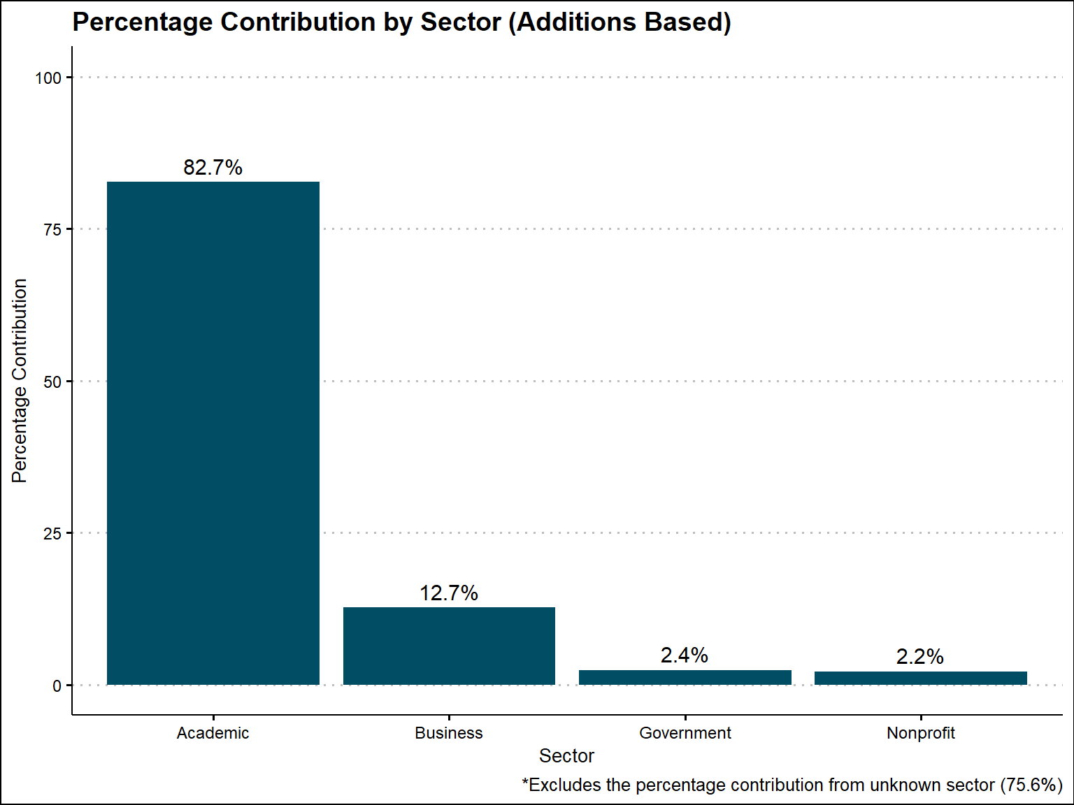

3.2 What is the distribution of GitHub R contributors by country?

The diverstidy function, which we use to extract country from a user, can supply some messy data in terms of identifying multiple countries for a unique user. We first need to clean that up before analyzing country distributions. There were 427 unique users that had multiple countries supplied, so we manually went through and decided whether all countries should be kept, or some should be deleted. The country extracted can be based on email, location, company, or an organization that a given user has listed.

Code

country_fix <- dbReadTable(con, "users_countries")

We filter out NA values here and replace with “Unknown”

Code

cran_users_unique <- cran_users_unique %>%
  mutate(
    country_fixed = strsplit(as.character(country), split = "\\|") %>%   # Split on "|"
      map(~unique(.)) %>%                                         # Keep only unique values
      sapply(paste, collapse = ",")                               # Collapse back into a string
  )

cran_users_unique <- cran_users_unique %>%
  mutate(country_fixed = ifelse(country_fixed == "NA", NA_character_, country_fixed))

cran_users_unique <- cran_users_unique %>%
  mutate(
    country_fixed = strsplit(country_fixed, split = ",") %>%  # Split on comma
      map(~ .[!. %in% "NA"]) %>%                             # Remove "NA" values (note the space before "NA")
      sapply(paste, collapse = ",")                           # Collapse back into a string
  )


cran_users_unique <- cran_users_unique %>%
                            left_join(country_fix, by = "login")

cran_users_unique <- cran_users_unique %>%
  mutate(country_final = ifelse(is.na(country_final), country_fixed, country_final))

cran_users_unique <- cran_users_unique %>%
  mutate(country_final = ifelse(is.na(country_final) | country_final == "NA", "Unknown", country_final))

Based on the unique R GitHub users, the United States is the most frequent country found followed by Germany and the United Kingdom. Out of 14,328 unique users, there were 5575 that we were unable to find a country for.

Code

### sum of Unknowns for country

sum(cran_users_unique$country_final == "Unknown")

[1] 5575

Code

### sorting to the top 10 most common countries for distinct GitHub users
top10_Countries_GitHub_users_unique <- cran_users_unique %>%
  filter(country_final != "Unknown")

top10_Countries_GitHub_users_unique <-  sort(table(top10_Countries_GitHub_users_unique$country_final), decreasing = T)

top10_Countries_GitHub_users_unique  <- as.data.frame(head(top10_Countries_GitHub_users_unique , 10))

colnames(top10_Countries_GitHub_users_unique ) <- c("country_final", "Freq")

 ### Graph output of top 10 countries for unique maintainers
 ggplot(top10_Countries_GitHub_users_unique , aes(x = reorder(country_final, Freq), y = Freq))+
   geom_bar(stat = "identity", fill = '#014d64') +
    coord_flip() +
    scale_y_continuous(expand = c(0,0)) +
    labs(x = "", y = "Number of GitHub Users",
         title = "Top 10 Countries for Unique R Users on GitHub" ) +
    ylim(c(0, 3000))+
  scale_fill_economist()+
  theme_clean()+
   theme(
  plot.title = element_text(size = 13))+
   labs(caption = "*Excludes count from unknown countries (5575)")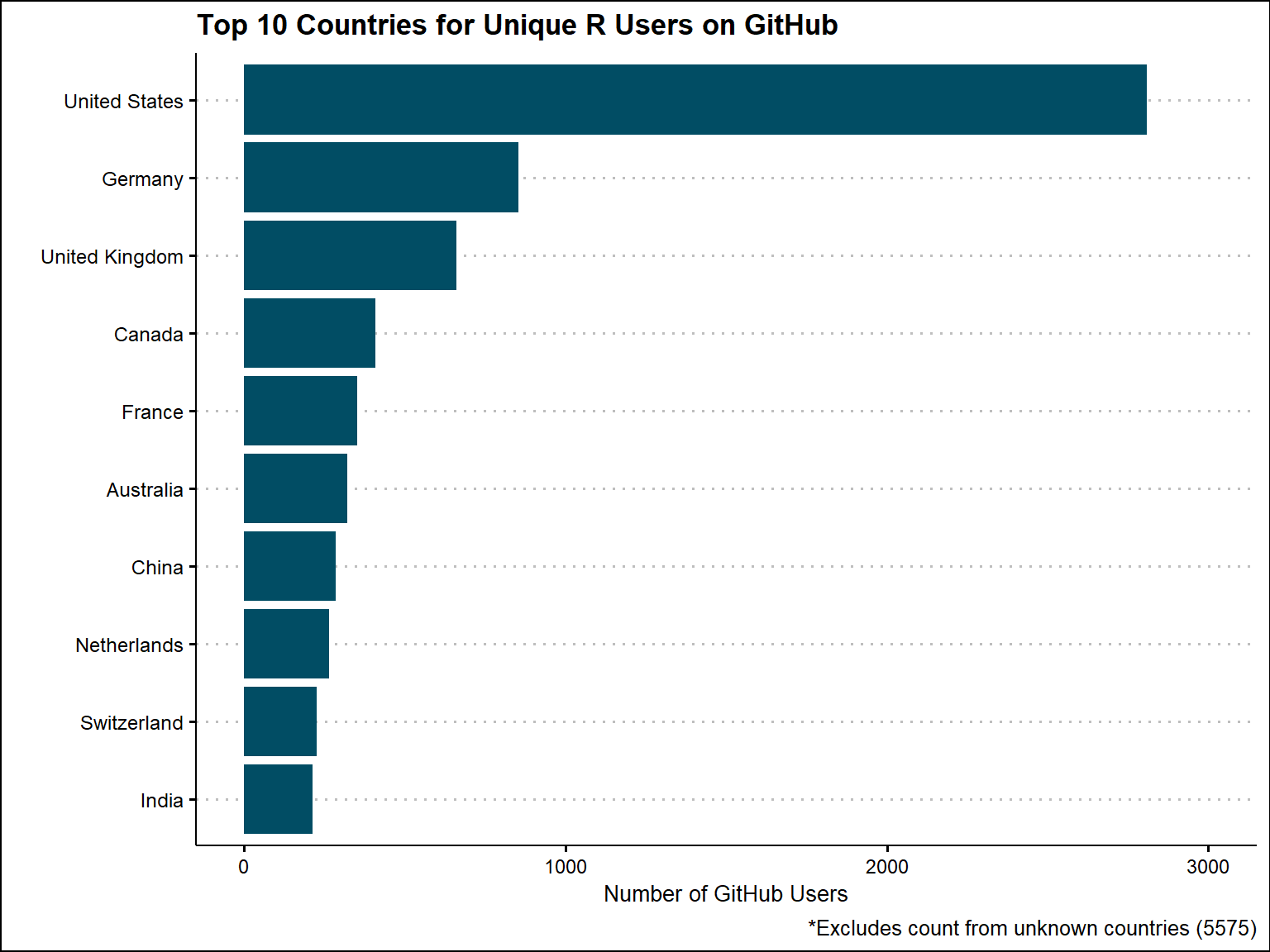

Code

### Table output of top 10 Institutions for packages
top10_Countries_GitHub_users_unique %>%
  kbl(caption = "Most Frequent Countries for R Developers on GitHub", escape = F)%>%
  kable_classic()%>%
  kable_styling(font_size = 12,  full_width = T)%>%
 row_spec(0, bold = T, background = '#014d64', color = "white")%>%
  column_spec(1:2, border_right = T)%>%
  scroll_box()

Most Frequent Countries for R Developers on GitHub

country_final	Freq
United States	2809
Germany	854
United Kingdom	660
Canada	410
France	352
Australia	322
China	286
Netherlands	264
Switzerland	226
India	214

3.2.1 How do we attribute contribution to countries (equal)?

As stated prior, there are some logins that have multiple countries listed. For these logins, we split the contribution fractions for equal and lines of code equally among the countries. So, if a user had two countries in a slug with 4 unique users, each country will get .125 credit based on equal contribution. For lines of code, if that user had 500 additions, each country would get 250 additions. After doing this, we see that there are 123 unique countries identified.

Code

# Function to handle the splitting and division for multiple countries
process_multiple_countries <- function(df) {
  num_countries <- length(str_split(df$country_final, ",\\s*")[[1]])
  df %>%
    separate_rows(country_final, sep = ",\\s*") %>%
    mutate(
      total_additions = total_additions / num_countries,
      contribution_fraction_equal = contribution_fraction_equal / num_countries,
      contribution_fraction_loc = contribution_fraction_loc / num_countries
    )
}

# join country variable back to commit table
user_countries <- cran_users_unique %>%
                    select(login, country_final)

user_commits_total <- user_commits_total %>%
                            left_join(user_countries, by = "login")

# Replace NA values in 'country_final' with 'Unknown'
user_commits_total$country_final[is.na(user_commits_total$country_final)] <- "Unknown"

# Process rows with multiple countries
multi_country_rows <- user_commits_total %>%
  filter(str_detect(country_final, ",")) %>%
  group_by(login) %>%
  do(process_multiple_countries(.))

# Exclude multi-country rows from the original df and bind the processed rows
user_commits_total <- user_commits_total %>%
  filter(!str_detect(country_final, ",")) %>%
  bind_rows(multi_country_rows)

Instead of grouping by sector, we have to group by country here.

Code

# Sum the contribution fraction for each sector per slug.
country_contribution <- user_commits_total %>%
  group_by(slug, country_final) %>%
  summarise(total_contribution_fraction = sum(contribution_fraction_equal))

# Aggregate the contribution fraction for each country across all slugs
country_aggregated <- country_contribution %>%
  group_by(country_final) %>%
  summarise(overall_contribution_fraction = sum(total_contribution_fraction))

# Calculate the total overall contribution fraction over all countries
total_overall_contribution = sum(country_aggregated$overall_contribution_fraction)

# Calculate the percentage contribution for each country
country_aggregated = country_aggregated %>%
  mutate(percentage_contribution = round((overall_contribution_fraction / total_overall_contribution) * 100, 1))

### Plot percentage contribution
country_aggregated$percentage_label <- scales::percent(country_aggregated$percentage_contribution / 100)

If we give equal contributions to countries, then the United states would get 31.1% of the credit followed by Germany with 10.9% credit. This excludes the contribution counted towards unknown (38.5%), so these percentages are based on the percentage that we know (61.5%).

Code

total_excluding_unknown <- sum(country_aggregated$overall_contribution_fraction[country_aggregated$country_final != "Unknown"])

country_aggregated <- country_aggregated %>%
  mutate(percentage_contribution_excl_unknown = ifelse(country_final != "Unknown", 
                                                       round((overall_contribution_fraction / total_excluding_unknown) * 100, 1), NA_real_))


country_aggregated$percentage_label_excl_unknown <- scales::percent(country_aggregated$percentage_contribution_excl_unknown / 100, accuracy = 0.1)


top_10_countries <- country_aggregated %>%
  arrange(desc(percentage_contribution_excl_unknown)) %>%
  head(10)

ggplot(top_10_countries, aes(x = reorder(country_final, percentage_contribution_excl_unknown),  y = percentage_contribution_excl_unknown)) +
  geom_bar(stat = "identity", fill = '#014d64') +
  geom_text(aes(label = percentage_label_excl_unknown), vjust = .5, size = 4, hjust = -.25) + # Adjust vjust and size as needed
  labs(title = "Percentage Contribution by Country (Equal Additions for Top 10 Countries)",
       x = "Country",
       y = "Percentage Contribution") +
  theme_clean() +
  ylim(0,100)+
  coord_flip()+
  theme(plot.title = element_text(size = 10))+
  labs(caption = "*Excludes the percentage contribution from unknown countries (38.5%)")

3.2.2 How do we attribute contribution to countries (additions)?

Now, we base the contribution on additions for country just as we did for sector.

Code

country_addition_contribution <- user_commits_total %>%
  group_by(slug, country_final) %>%
  summarise(total_addition_contribution = sum(contribution_fraction_loc))

country_aggregated_additions <- country_addition_contribution %>%
  group_by(country_final) %>%
  summarise(overall_addition_contribution = sum(total_addition_contribution, na.rm = TRUE))

total_overall_additions = sum(country_aggregated_additions$overall_addition_contribution)

country_aggregated_additions$percentage_additions = round((country_aggregated_additions$overall_addition_contribution / total_overall_additions) * 100,1)

country_aggregated_additions$percentage_label_additions = scales::percent(country_aggregated_additions$percentage_additions / 100)

Based on additions, the percentage attributed towards unknwon decreases to 34.1%, so the percentage that we know increases to 65.9% overall. United states still is at the top, but it decreases slightly to 30.9%. The top 10 and the order of the top 10 stays the same, but the percentages increase slightly for the ones more towards the bottom.

Code

total_excluding_unknown <- sum(country_aggregated_additions$overall_addition_contribution[country_aggregated_additions$country_final != "Unknown"])

country_aggregated_additions <- country_aggregated_additions %>%
  mutate(percentage_contribution_excl_unknown = ifelse(country_final != "Unknown", 
                                                       round((overall_addition_contribution / total_excluding_unknown) * 100, 1), NA_real_))


country_aggregated_additions$percentage_label_excl_unknown <- scales::percent(country_aggregated_additions$percentage_contribution_excl_unknown / 100, accuracy = 0.1)


top_10_countries_additions <- country_aggregated_additions %>%
  arrange(desc(percentage_contribution_excl_unknown)) %>%
  head(10)

ggplot(top_10_countries_additions, aes(x = reorder(country_final, percentage_contribution_excl_unknown),  y = percentage_contribution_excl_unknown)) +
  geom_bar(stat = "identity", fill = '#014d64') +
  geom_text(aes(label = percentage_label_excl_unknown), vjust = .5, size = 4, hjust = -.25) + # Adjust vjust and size as needed
  labs(title = "Percentage Contribution by Country (Equal Additions for Top 10 Countries)",
       x = "Country",
       y = "Percentage Contribution") +
  theme_clean() +
  ylim(0,100)+
  coord_flip()+
  theme(plot.title = element_text(size = 10))+
  labs(caption = "*Excludes the percentage contribution from unknown (34.1%)")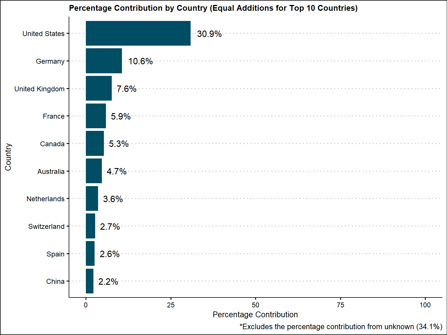

3.3 What is the distribution of unique GitHub R contributors by organization?

We also have the organization variable for some users. It works with the sector variable, so if we were not able to identify a sector, we also were not able to identify an organization.

Code

# Replace NA values in 'organization' with 'Unknown'
user_commits_total$organization[is.na(user_commits_total$organization)] <- "Unknown"

If we look at the top 10 most frequent organizations for unique R developers on Github, Google has the most with 86 followed by NetEase with 57. Only one in the top 10 is from a sector other than business or academic (Broad Institute - nonprofit)

Code

### sorting to the top 10 most common institutions for distinct GitHub users
top10_Institutions_GitHub_users_unique <- sort(table(cran_users_unique$organization), decreasing = T)
top10_Institutions_GitHub_users_unique <- as.data.frame(head(top10_Institutions_GitHub_users_unique, 10))

colnames(top10_Institutions_GitHub_users_unique) <- c("organization", "Freq")

### joining to institution unique dataframe to get sector variable
top10_Institutions_GitHub_users_unique <- cran_users_unique %>% 
  right_join(top10_Institutions_GitHub_users_unique, by = "organization")%>%
  distinct(organization, .keep_all = T)%>%
  select(organization, sector, Freq)%>%
  arrange(desc(Freq))

 ### Graph output of top 10 institutions for unique maintainers
 ggplot(top10_Institutions_GitHub_users_unique, aes(x = reorder(organization, Freq), y = Freq, fill = sector))+
   geom_bar(stat = "identity") +
    coord_flip() +
    scale_y_continuous(expand = c(0,0)) +
    labs(x = "", y = "Number of GitHub Users",
         title = "Top 10 Institutions for Unique Users on GitHub" ) +
    ylim(c(0, 200))+
  scale_fill_economist()+
  theme_clean()+
   theme(
  plot.title = element_text(size = 13))+
   labs(caption = "*Those without organization information are removed in this figure (82% of 14,328 R Developers)")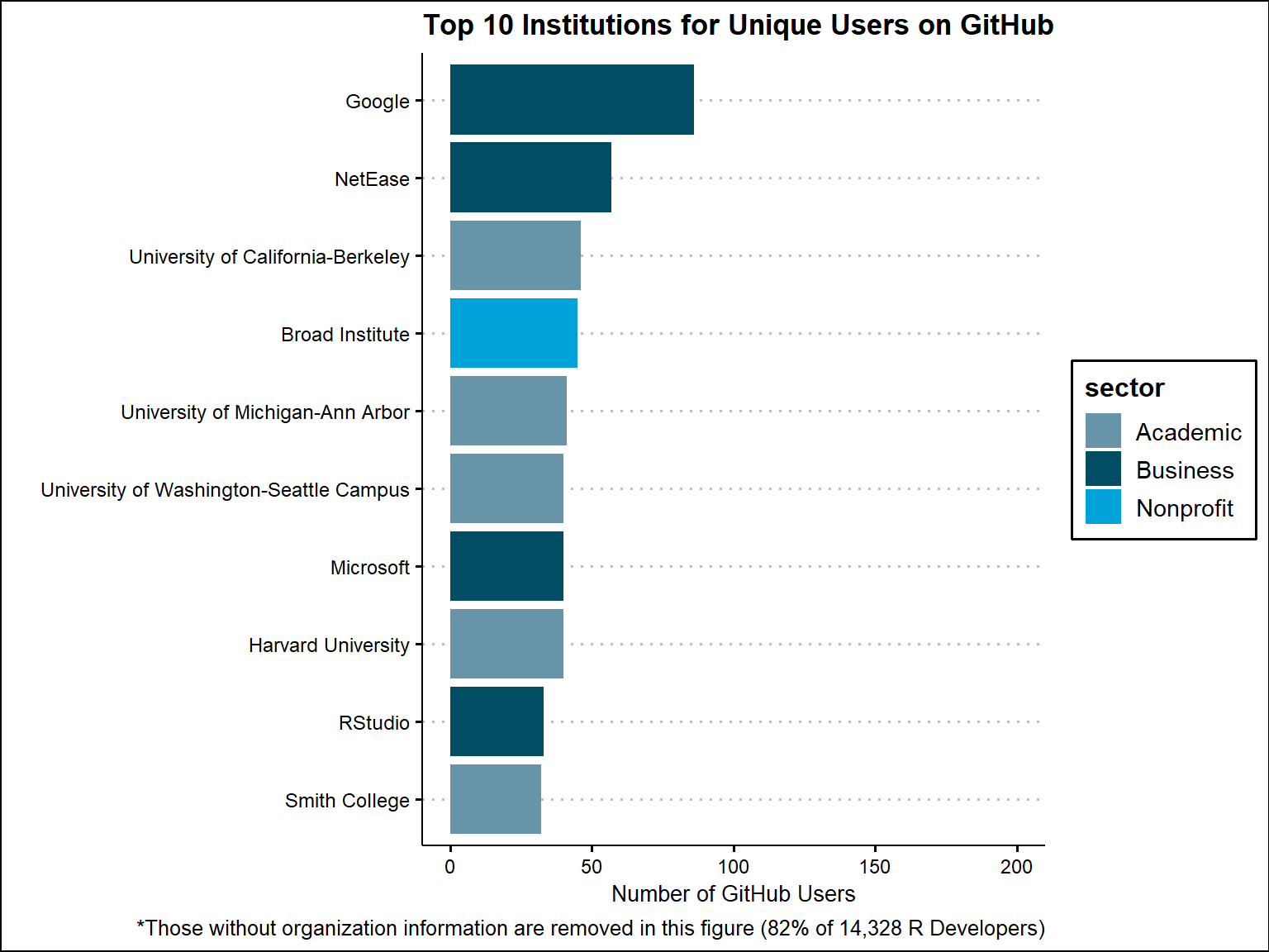

Code

### Table output of top 10 Institutions for packages
top10_Institutions_GitHub_users_unique %>%
  kbl(caption = "Most Frequent Institutions for R Developers on GitHub", escape = F)%>%
  kable_classic()%>%
  kable_styling(font_size = 12,  full_width = T)%>%
 row_spec(0, bold = T, background = '#014d64', color = "white")%>%
  column_spec(1:2, border_right = T)%>%
  scroll_box()

Most Frequent Institutions for R Developers on GitHub

organization	sector	Freq
Google	Business	86
NetEase	Business	57
University of California-Berkeley	Academic	46
Broad Institute	Nonprofit	45
University of Michigan-Ann Arbor	Academic	41
University of Washington-Seattle Campus	Academic	40
Harvard University	Academic	40
Microsoft	Business	40
RStudio	Business	33
Smith College	Academic	32

3.3.1 How do we attribute contribution to organization (equal)?

We now will look at equal contribution for organizations

Code

# Sum the contribution fraction for each organization per slug.
org_contribution <- user_commits_total %>%
  group_by(slug, organization) %>%
  summarise(total_contribution_fraction = sum(contribution_fraction_equal))

# Aggregate the contribution fraction for organization across all slugs
org_aggregated <- org_contribution %>%
  group_by(organization) %>%
  summarise(overall_contribution_fraction = sum(total_contribution_fraction))

# Calculate the total overall contribution fraction over all organizations
total_overall_contribution = sum(org_aggregated$overall_contribution_fraction)

# Calculate the percentage contribution for each organization
org_aggregated = org_aggregated %>%
  mutate(percentage_contribution = round((overall_contribution_fraction / total_overall_contribution) * 100, 1))

### Plot percentage contribution
org_aggregated$percentage_label <- scales::percent(org_aggregated$percentage_contribution / 100)

Again, the equal percentage contribution to Unknown is 77.7% just like we saw in the sector contribution section. Of the percentage we do know (611 different organizations), Rstudio leads with 7.2% followed by UCLA with 3%

Code

total_excluding_unknown <- sum(org_aggregated$overall_contribution_fraction[org_aggregated$organization != "Unknown"])

org_aggregated <- org_aggregated %>%
  mutate(percentage_contribution_excl_unknown = ifelse(organization != "Unknown", 
                                                       round((overall_contribution_fraction / total_excluding_unknown) * 100, 1), NA_real_))


org_aggregated$percentage_label_excl_unknown <- scales::percent(org_aggregated$percentage_contribution_excl_unknown / 100, accuracy = 0.1)


top_10_orgs <- org_aggregated %>%
  arrange(desc(percentage_contribution_excl_unknown)) %>%
  head(10)

ggplot(top_10_orgs, aes(x = reorder(organization, percentage_contribution_excl_unknown),  y = percentage_contribution_excl_unknown)) +
  geom_bar(stat = "identity", fill = '#014d64') +
  geom_text(aes(label = percentage_label_excl_unknown), vjust = .5, size = 4, hjust = -.25) + # Adjust vjust and size as needed
  labs(title = "Percentage Contribution by Organization (Equal Contribution for Top 10 Organizations)",
       x = "Organization",
       y = "Percentage Contribution") +
  theme_clean() +
  ylim(0,100)+
  coord_flip()+
  theme(plot.title = element_text(size = 7))+
  labs(caption = "*Excludes the percentage contribution from unknown organizations (77.7%)")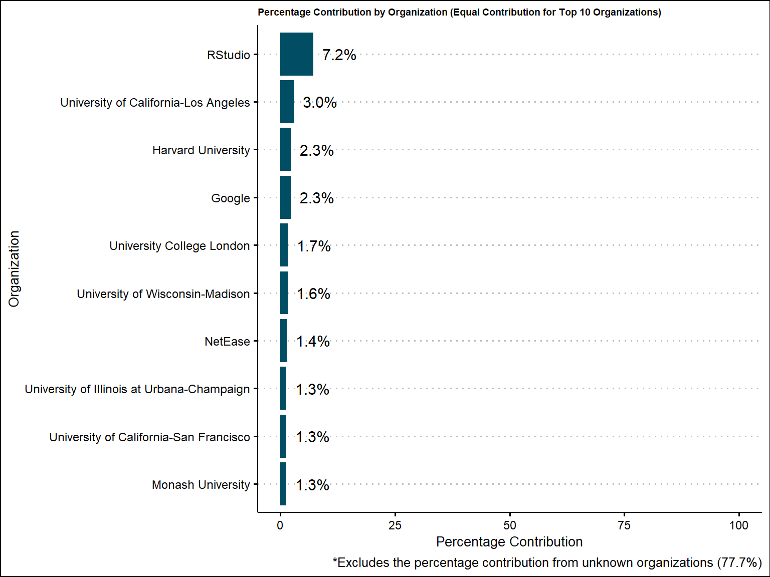

3.3.2 How do we attribute contribution to organizations (additions based)?

Now, we base the contribution on additions for organization just as we did for sector and country.

Code

org_addition_contribution <- user_commits_total %>%
  group_by(slug, organization) %>%
  summarise(total_addition_contribution = sum(contribution_fraction_loc))

org_aggregated_additions <- org_addition_contribution %>%
  group_by(organization) %>%
  summarise(overall_addition_contribution = sum(total_addition_contribution, na.rm = TRUE))

total_overall_additions = sum(org_aggregated_additions$overall_addition_contribution)

org_aggregated_additions$percentage_additions = round((org_aggregated_additions$overall_addition_contribution / total_overall_additions) * 100,1)

org_aggregated_additions$percentage_label_additions = scales::percent(org_aggregated_additions$percentage_additions / 100)

Based on additions, the percentage contribution towards unknown is 75.6% just as we saw for sector, which is what we expect because the two variables coincide with one another. The percentage coming from Rstudio decreases to 5.9% (still number one), and the top 10 along with the order of the top 10 changes slightly. Notably, Monash University moves from the 10th position to the 4th position when factoring in additions.

Code

total_excluding_unknown <- sum(org_aggregated_additions$overall_addition_contribution[org_aggregated_additions$organization != "Unknown"])

org_aggregated_additions <- org_aggregated_additions %>%
  mutate(percentage_contribution_excl_unknown = ifelse(organization != "Unknown", 
                                                       round((overall_addition_contribution / total_excluding_unknown) * 100, 1), NA_real_))


org_aggregated_additions$percentage_label_excl_unknown <- scales::percent(org_aggregated_additions$percentage_contribution_excl_unknown / 100, accuracy = 0.1)


top_10_orgs_additions <- org_aggregated_additions %>%
  arrange(desc(percentage_contribution_excl_unknown)) %>%
  head(10)

ggplot(top_10_orgs_additions, aes(x = reorder(organization, percentage_contribution_excl_unknown),  y = percentage_contribution_excl_unknown)) +
  geom_bar(stat = "identity", fill = '#014d64') +
  geom_text(aes(label = percentage_label_excl_unknown), vjust = .5, size = 4, hjust = -.25) + # Adjust vjust and size as needed
  labs(title = "Percentage Contribution by Organization (Additions Based Contribution for Top 10 Organizations)",
       x = "Organization",
       y = "Percentage Contribution") +
  theme_clean() +
  ylim(0,100)+
  coord_flip()+
  theme(plot.title = element_text(size = 7))+
  labs(caption = "*Excludes the percentage contribution from unknown (75.6%)")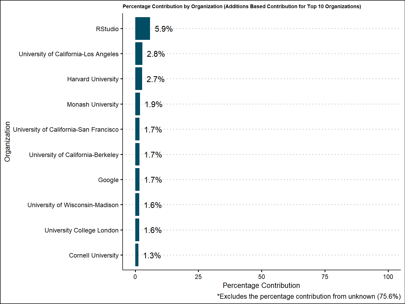

2. Network Analysis

• What are the overall structural features of the OSS networks? How do they differ across fields, sectors, institutions, and countries? Units of analysis (OSS actors): projects, categories, developers, institutions, sectors, countries

• What are the different communities that can be identified using structural features of the networks? Do they correspond to similarities in languages, methods, location, culture?

Code

#### CReate edge list for reverse dependencies


cran_github_edge <- cran_github %>%
                      select(Package, Maintainer, Maintainer_Name, slug, Reverse_Depends, Reverse_Depends_Count, Sector, Institution)

cran_github_edge$Package_Dependent <- cran_github_edge$Reverse_Depends


cran_github_edge <- cran_github_edge %>%
                      full_join(user_commits_total, by = "slug")%>%
                        select(Package, slug, Reverse_Depends, Reverse_Depends_Count, login, name,
                             country_final, total_additions, total_code_for_slug, Package_Dependent) %>%
                       # Remove rows with NA in Depends
                        filter(!is.na(Package_Dependent))



colnames(cran_github_edge) <- c("Package", "Slug", "Reverse_Depends", "Reverse_Depends_Count",
                                "Parent_Contributor_Login", "Parent_Contributor_Name", "Parent_Contributor_Country",
                                "Parent_Contributor_Additions", "Parent_Total_Slug_Additions", "Package_Dependent")


#### transform to long
cran_github_edge_network <-  cran_github_edge %>%
  # Separate rows
  separate_rows(Package_Dependent, sep = ",\\s*")

#### create dataframe for dependent packages to join dependent contributor information
user_commits_edge <- user_commits_total %>%
  mutate(Package_Dependent = str_split(slug, "/", simplify = TRUE)[, 2])%>%
  select(login, name, country_final, total_additions, total_code_for_slug, Package_Dependent)
  
  colnames(user_commits_edge) <- c("Dependent_Contributor_Name", "Dependent_Contributor_Login", "Dependent_Contributor_Country", 
                                   "Dependent_Contributor_Additions", "Dependent_Total_Slug_Additions", "Package_Dependent")
  
  ### join contributors from dependent package
  cran_github_edge_network_full <- cran_github_edge_network %>%
                                        left_join(user_commits_edge, by = "Package_Dependent")

Code

cran_github_edge_network_full$Parent_Contributor_Fraction <- cran_github_edge_network_full$Parent_Contributor_Additions/ cran_github_edge_network_full$Parent_Total_Slug_Additions


cran_github_edge_network_full_test <- cran_github_edge_network_full %>%
                                          select(Parent_Contributor_Country, Dependent_Contributor_Country, Parent_Contributor_Fraction)

head(cran_github_edge_network_full_test)

3. Measuring Impact: OSS Developers and Projects

• Who are the key players (projects, developers, institutions, sectors, and countries) on the networks and how has this changed over time?

• How do the positions of OSS actors impact OSS contributions?

4. Diffusion of Open Source Software Innovation

• What are the major paths from/to countries, sectors, institutions and fields that OSS innovation disseminates?

• What are the upstream and downstream actors, i.e., sectors, institutions, and countries?