Code.gov

Code.gov is the Federal Government’s platform for sharing and open sourcing software from Government Agencies. Recent policies of the U.S. Federal Government such as the Federal Source Code Policy (FSCP) promote the sharing of software source code developed by or for the Federal Government. Public funding for creation of software by or for the Federal Government and for research through universities plays an important role but it is not fully accounted. Our aim is to measure how much of OSS is developed in the U.S. Federal Government and estimate its value. As OSS is disseminated online, a wealth of information is available in the code and source code repositories of the software programs themselves. Examples include: contributors, their organizations, lines of code contributed, etc. We use non-survey data from Code.gov which is the Federal Government’s platform for sharing and open sourcing software from Government Agencies.

Objectives

Our aim is to measure how much of OSS is developed in the U.S. Federal Government and estimate its value. This page below provides insights from Exploratory Data Analysis

Data and Methods

The data acquired from Code.gov is in JSON format covering over 17,000 software projects, across 21 different Federal Agencies and includes information on each project, agency name, host links, descriptions and other information. Most of these are developed and hosted on GitHub. We also use GitHub to obtain related information.

Our second source of data is GitHub – a popular version control and hosting service which is the largest platform in the world with over 108 million users and 100 million public repositories. From GitHub we have collected data on over 7.8 million repositories, 2.1 million users and 778 million commits. The information gathered from GitHub includes commits, lines of code added and deleted, OSI licenses, users’ login information, organization, locations, emails, etc.

Exploratory Data Analysis

Add text here

Hosting Platforms

Code

# establishing connection and listing all tables in database
con <- dbConnect(MySQL(), user = Sys.getenv("DB_USERNAME"), password = Sys.getenv("DB_PASSWORD"),
    dbname = "codegov", host = "oss-1.cij9gk1eehyr.us-east-1.rds.amazonaws.com")

hosting <- dbReadTable(con, "codegov_agency_hosting")

dbDisconnect(con)

[1] TRUE

Code

hosting <- hosting |>
  mutate(total_hosting = rowSums(across(where(is.numeric)))) |>
  select(domain, total_hosting) |>
  filter(!row_number() %in% c(10))



#theme_set(theme_wes())
  

hosting |>
  mutate(domain = fct_reorder(domain, total_hosting)) |>
  ggplot(aes(x = domain, y = total_hosting)) + 
    geom_bar(stat = "identity", fill = '#014d64', width=.6) +
    coord_flip() +
    theme(legend.title=element_blank()) +
    labs(title = "Hosting Platforms by Projects Hosted",
         subtitle = "Github is the most popular hosting platform",
        x = "Hosting Platform",
        y = "Count of Projects")

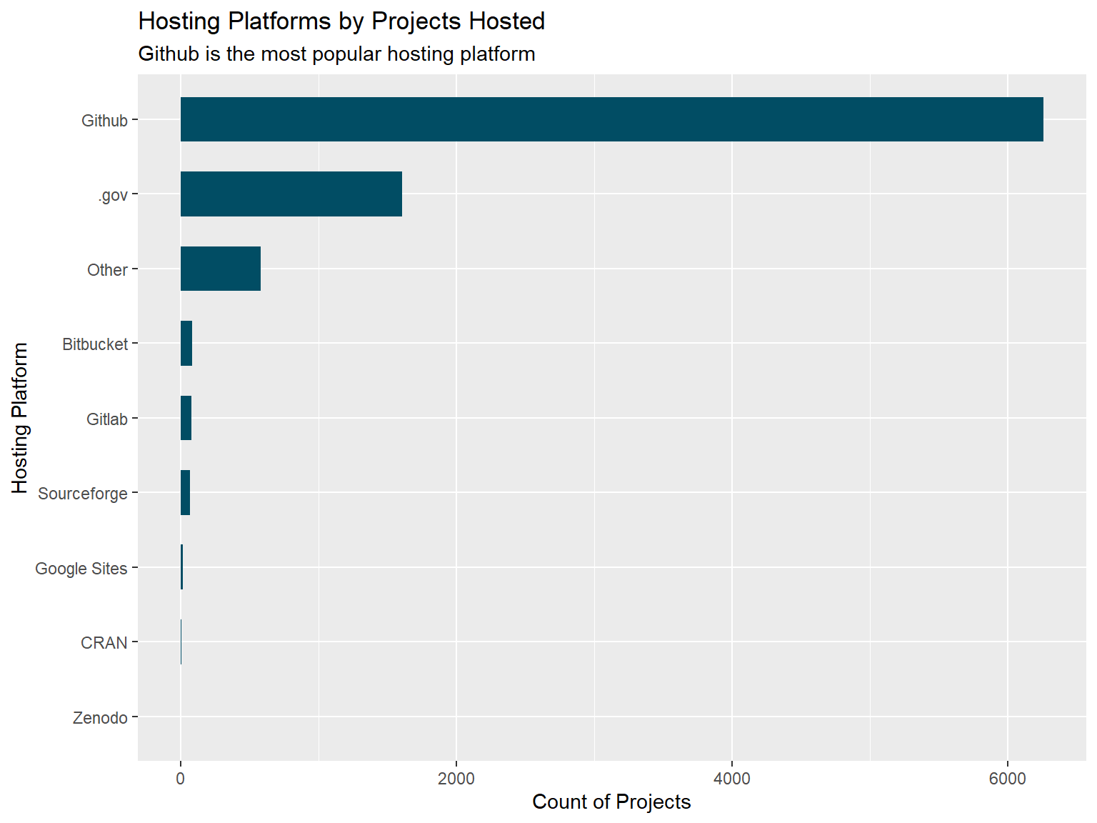
The most popular hosting platform for Code.gov projects is GitHub followed by the Code.gov platform itself.

Government Agencies

Code

# establishing connection and listing all tables in database
con <- dbConnect(MySQL(), user = Sys.getenv("DB_USERNAME"), password = Sys.getenv("DB_PASSWORD"),
    dbname = "codegov", host = "oss-1.cij9gk1eehyr.us-east-1.rds.amazonaws.com")

agency <- dbReadTable(con, "codegov_gh_agency_count")

dbDisconnect(con)

[1] TRUE

Code

agency |>
  select(agency, projects) |>
  mutate(agency = fct_reorder(agency, projects)) |>
  ggplot(aes(x = agency, y = projects)) +
    geom_bar(stat = "identity", fill = '#014d64', width=.6) +
    coord_flip() +
    theme(legend.title=element_blank()) +
    labs(title = "Number of Projects by Agency",
        x = "",
        y = "Count of Projects")

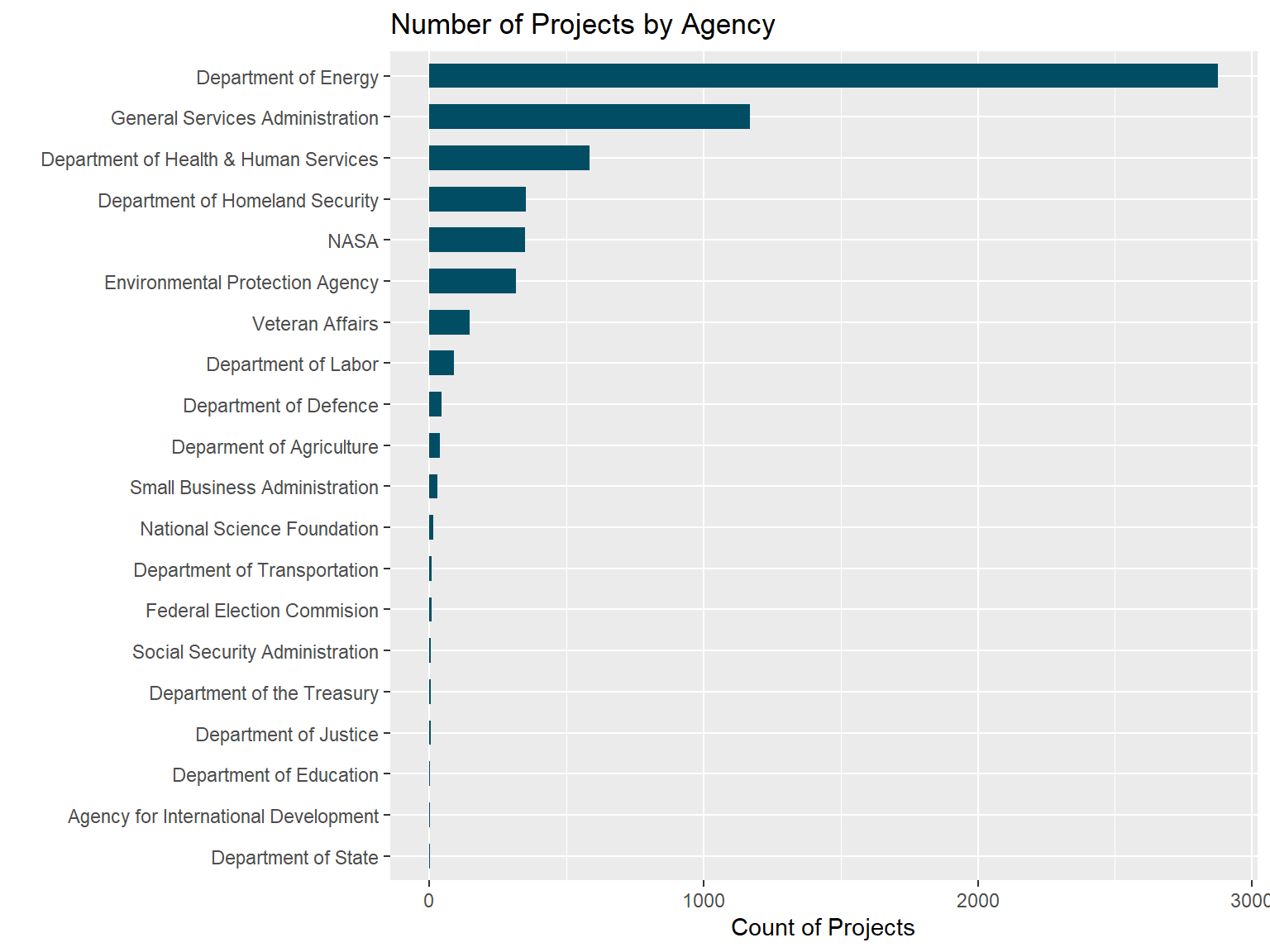
The Department of Energy, the General Services Administration and the Department of Health & Human Services are the top 3 agencies by number of projects showcased on the Code.gov platform.

Contributing Sectors

Code

# establishing connection and listing all tables in database
con <- dbConnect(MySQL(), user = Sys.getenv("DB_USERNAME"), password = Sys.getenv("DB_PASSWORD"),
    dbname = "codegov", host = "oss-1.cij9gk1eehyr.us-east-1.rds.amazonaws.com")

sectors <- dbReadTable(con, "codegov_users_sectored")

dbDisconnect(con)

[1] TRUE

Code

sectors_count <- sectors |>
  summarise(Academic = sum(academic, na.rm = T),
            Business = sum(business, na.rm = T),
            Government = sum(government,  na.rm = T),
            `Non-Profit` = sum(nonprofit, na.rm = T))

sectors_count <- sectors_count |>
  gather(key = "Sectors", value = "Contributors")
  
ggplot(sectors_count, aes(area = Contributors, fill = Sectors, label = Contributors)) +
  geom_treemap() +
  geom_treemap_text(colour = "black",
                    place = "centre",
                    size = 15)+
  ggtitle("Number of Contributors Per Sector")+
  scale_fill_economist()

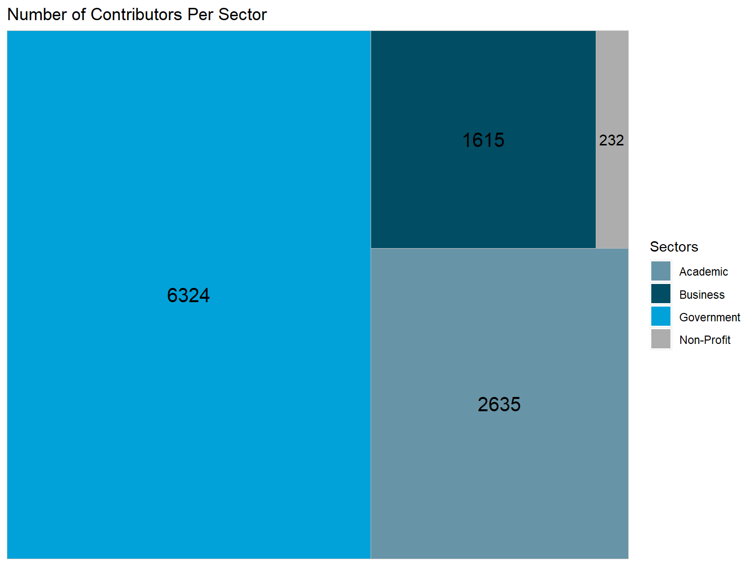
Contributors belonging to the Government sector were the highest with 6,324 contributors followed by the Academic sector with 2,635 contributors, Business sector with 1,615 contributors and the Non-Profit sector with 232 contributors.

Top 20 Organizations By Number of Contributors

Code

# establishing connection and listing all tables in database
con <- dbConnect(MySQL(), user = Sys.getenv("DB_USERNAME"), password = Sys.getenv("DB_PASSWORD"),
    dbname = "codegov", host = "oss-1.cij9gk1eehyr.us-east-1.rds.amazonaws.com")

users <- dbReadTable(con, "codegov_users_sectors")

dbDisconnect(con)

[1] TRUE

Code

orgs_count <- users |>
  count(organization, name = 'Contributors', sort = T) |>
  rename(Organization = organization) |>
  arrange(desc(Contributors)) |>
  top_n(21, Contributors) |>
  slice(2:21)

orgs_count |>
  select(Organization, Contributors) |>
  mutate(Organization = fct_reorder(Organization, Contributors)) |>
  ggplot(aes(x = Organization, y = Contributors)) +
    geom_bar(stat = "identity", fill = '#014d64', width=.6) +
    coord_flip() +
   geom_text(aes(label=Contributors), color='white', position=position_dodge(width = 0.05), hjust=1.2, size = 7/.pt) +
    theme(legend.title=element_blank()) +
    labs(title = "Number of Contributors by Organization",
        x = "",
        y = "Count of Contributors")

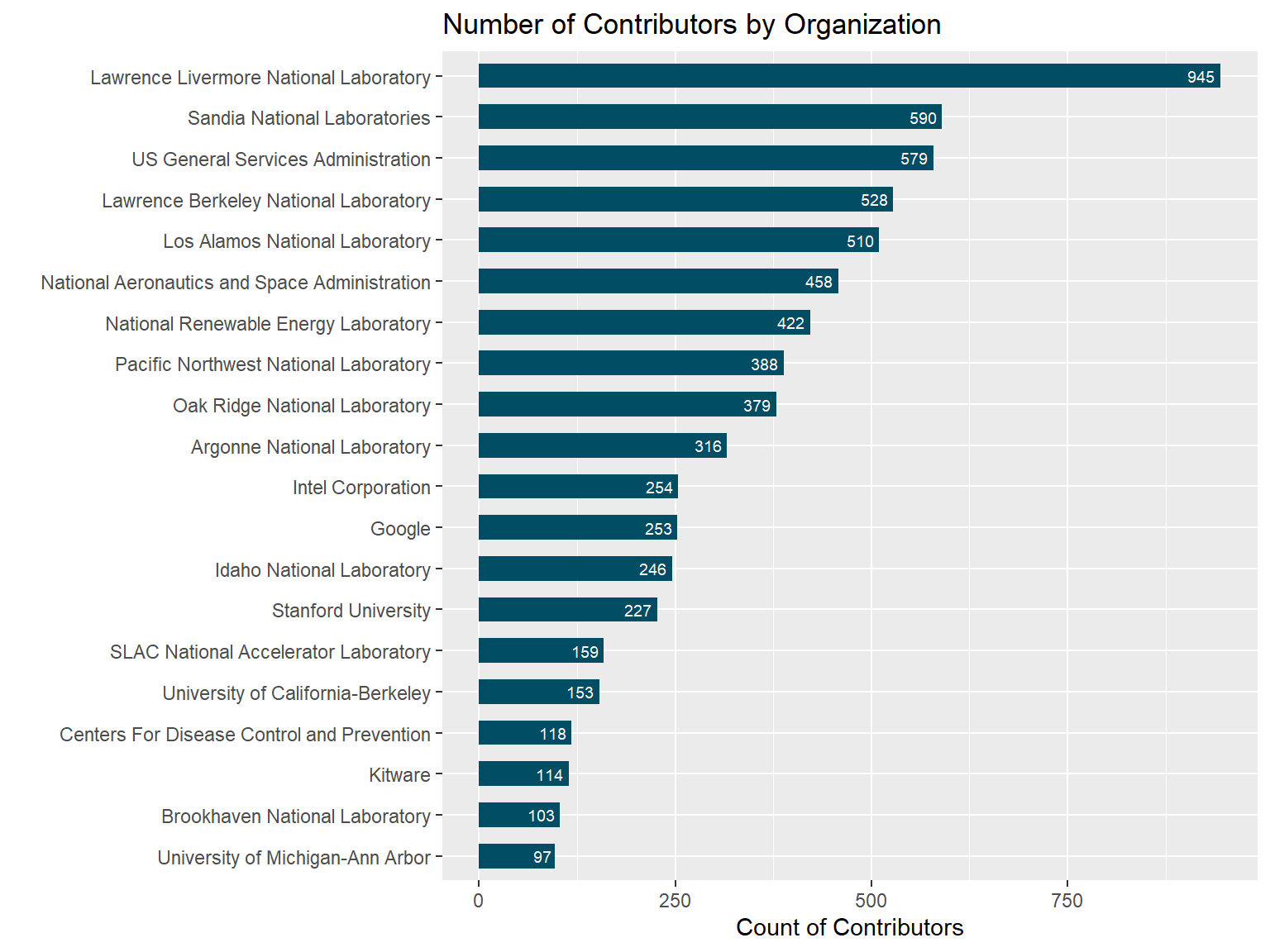
The highest number of contributors by organizations were the Lawrence Livermore National Laboratory and Sandia National Laboratory. Private sector organizations with the highest number of contributors were Intel Corporation and Google.

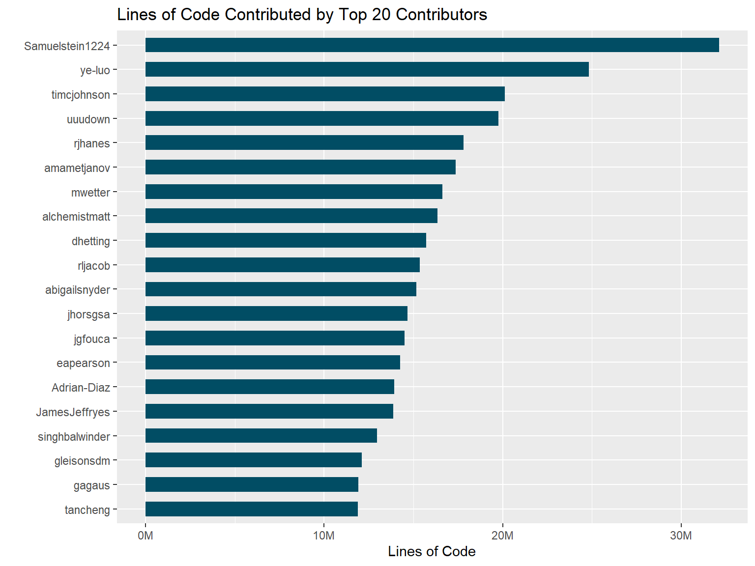
Top 20 Contributors by Lines of Code Added

Code

#establishing connection and listing all tables in database
con <- dbConnect(MySQL(), user = Sys.getenv("DB_USERNAME"), password = Sys.getenv("DB_PASSWORD"),
    dbname = "codegov", host = "oss-1.cij9gk1eehyr.us-east-1.rds.amazonaws.com")

contri <- dbReadTable(con, "codegov_gh_commits_by_login")

dbDisconnect(con)

[1] TRUE

Code

cont_count <- contri |>
  select(login, additions) |>
  group_by(login) |>
  summarise(Contribution = sum(additions)) |>
  rename(Contributor = login) |>
  arrange(desc(Contribution)) |>
  top_n(20, Contribution)

cont_count |>
  select(Contributor, Contribution) |>
  mutate(Contributor = fct_reorder(Contributor, Contribution)) |>
  ggplot(aes(x = Contributor, y = Contribution)) +
    geom_bar(stat = "identity", fill = '#014d64', width=.6) +
    scale_y_continuous(labels = label_number(suffix = "M", scale = 1e-6, big.mark = ",")) +
    coord_flip() +
    theme(legend.title=element_blank()) +
    labs(title = "Lines of Code Contributed by Top 20 Contributors",
        x = "",
        y = "Lines of Code")

Detailed Info of Top 20 Contributors (Table)

Code

top_20_users <- cont_count %>%
  left_join(users, by = join_by(Contributor == login)) |>
  group_by(Contributor) |>
  filter(row_number()==1)


top_20_users

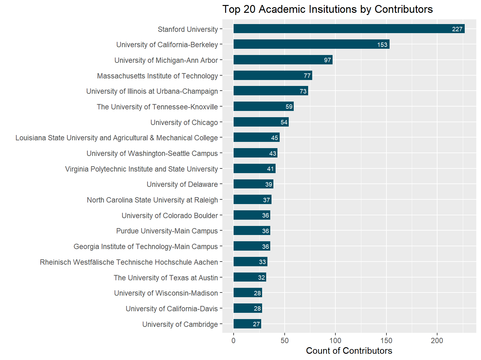
Top 20 Academic Institutions By Number of Contributors

Code

# establishing connection and listing all tables in database
con <- dbConnect(MySQL(), user = Sys.getenv("DB_USERNAME"), password = Sys.getenv("DB_PASSWORD"),
    dbname = "codegov", host = "oss-1.cij9gk1eehyr.us-east-1.rds.amazonaws.com")

users <- dbReadTable(con, "codegov_users_sectors")

dbDisconnect(con)

[1] TRUE

Code

orgs_count <- users |>
  filter(sector == 'Academic') |>
  count(organization, name = 'Contributors', sort = T) |>
  rename(Organization = organization) |>
  arrange(desc(Contributors)) |>
  top_n(20, Contributors)

orgs_count |>
  select(Organization, Contributors) |>
  mutate(Organization = fct_reorder(Organization, Contributors)) |>
  ggplot(aes(x = Organization, y = Contributors)) +
    geom_bar(stat = "identity", fill = '#014d64', width=.6) +
    coord_flip() +
    geom_text(aes(label=Contributors), color='white', position=position_dodge(width = 0.05), hjust=1.2, size = 7/.pt) +
    theme(legend.title=element_blank()) +
    labs(title = "Top 20 Academic Insitutions by Contributors",
        x = "",
        y = "Count of Contributors")

Stanford University is the academic institution with the highest number of contributors followed by University of California - Berkeley and University of Michigan - Ann Arbor.

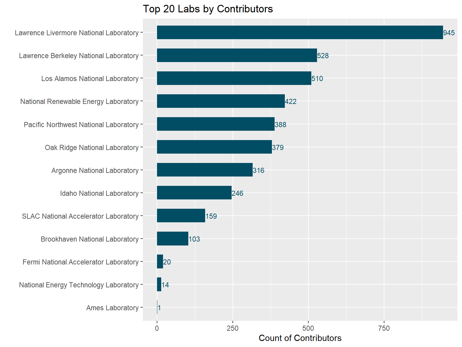
Top 20 Contributing Research Labs

Code

# establishing connection and listing all tables in database
con <- dbConnect(MySQL(), user = Sys.getenv("DB_USERNAME"), password = Sys.getenv("DB_PASSWORD"),
    dbname = "codegov", host = "oss-1.cij9gk1eehyr.us-east-1.rds.amazonaws.com")

users <- dbReadTable(con, "codegov_users_sectors")

dbDisconnect(con)

[1] TRUE

Code

orgs_count <- users |>
  filter(grepl('Laboratory', organization)) |>
  count(organization, name = 'Contributors', sort = T) |>
  rename(Organization = organization) |>
  arrange(desc(Contributors)) |>
  top_n(20, Contributors)

orgs_count |>
  select(Organization, Contributors) |>
  mutate(Organization = fct_reorder(Organization, Contributors)) |>
  ggplot(aes(x = Organization, y = Contributors)) +
    geom_bar(stat = "identity", fill = '#014d64', width=.6) +
    geom_text(aes(label=Contributors), color='#014d64', position=position_dodge(width=0.5), hjust=-0, size = 9/.pt) +
    coord_flip() +
    theme(legend.title=element_blank()) +
    labs(title = "Top 20 Labs by Contributors",
        x = "",
        y = "Count of Contributors")

The Lawrence Livermore National Laboratory is has the highest number of contributors out of all Laboratories.

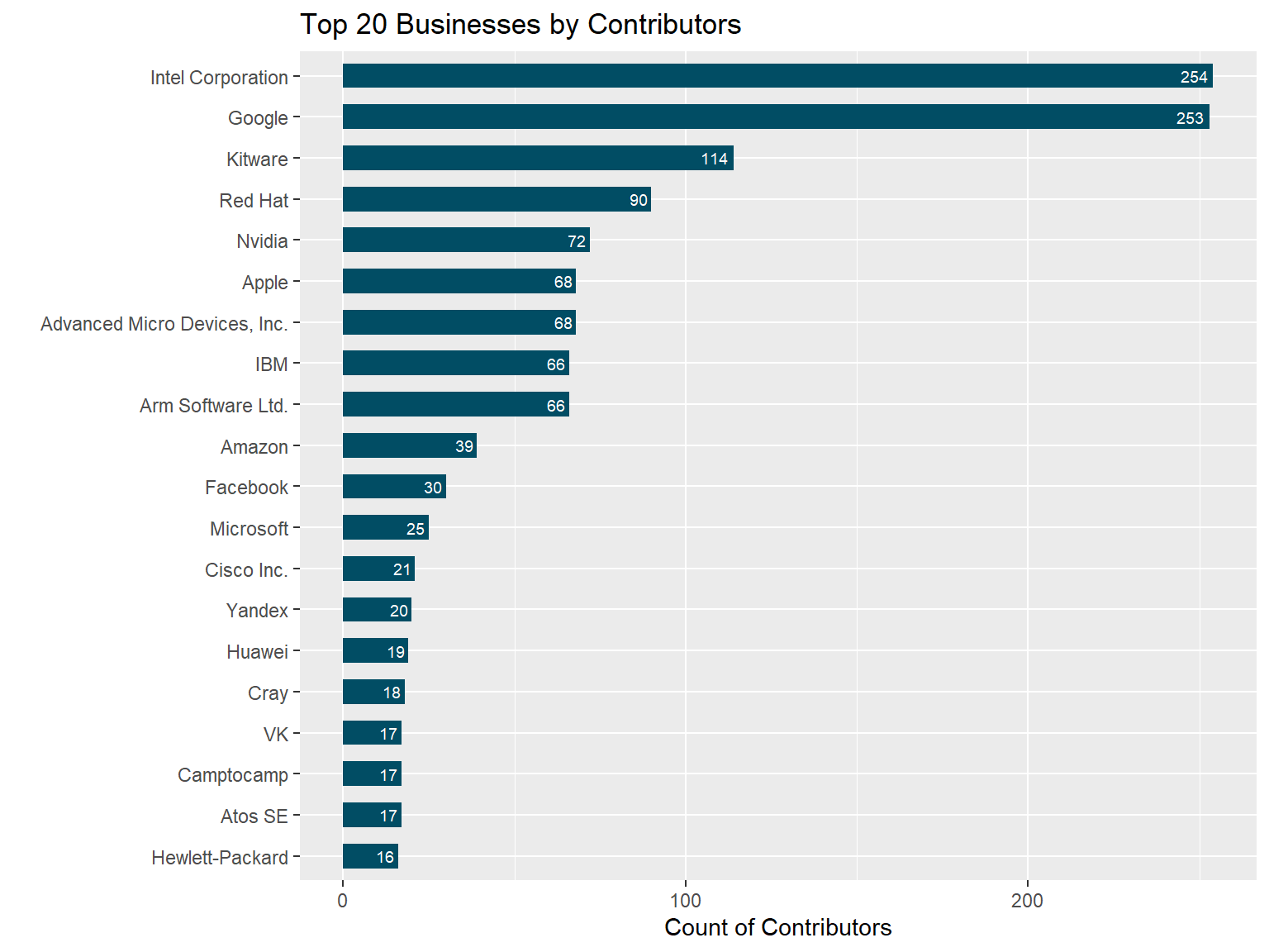
Top 20 Contributing Businesses

Code

# establishing connection and listing all tables in database
con <- dbConnect(MySQL(), user = Sys.getenv("DB_USERNAME"), password = Sys.getenv("DB_PASSWORD"),
    dbname = "codegov", host = "oss-1.cij9gk1eehyr.us-east-1.rds.amazonaws.com")

users <- dbReadTable(con, "codegov_users_sectors")

dbDisconnect(con)

[1] TRUE

Code

orgs_count <- users |>
  filter(sector == 'Business') |>
  count(organization, name = 'Contributors', sort = T) |>
  rename(Organization = organization) |>
  arrange(desc(Contributors)) |>
  top_n(20, Contributors)

orgs_count |>
  select(Organization, Contributors) |>
  mutate(Organization = fct_reorder(Organization, Contributors)) |>
  ggplot(aes(x = Organization, y = Contributors)) +
    geom_bar(stat = "identity", fill = '#014d64', width=.6) +
    coord_flip() +
    geom_text(aes(label=Contributors), color='white', position=position_dodge(width = 0.05), hjust=1.2, size = 7/.pt) +
    theme(legend.title=element_blank()) +
    labs(title = "Top 20 Businesses by Contributors",
        x = "",
        y = "Count of Contributors")

Intel Corporation, Google and Kitware are the top 3 corporations with the highest number of contributors.

Cost Calculations

Code

# establishing connection and listing all tables in database
con <- dbConnect(MySQL(), user = Sys.getenv("DB_USERNAME"), password = Sys.getenv("DB_PASSWORD"),
    dbname = "codegov", host = "oss-1.cij9gk1eehyr.us-east-1.rds.amazonaws.com")

counts_repo <- dbReadTable(con, "codegov_gh_commits_by_agency")

dbDisconnect(con)

[1] TRUE

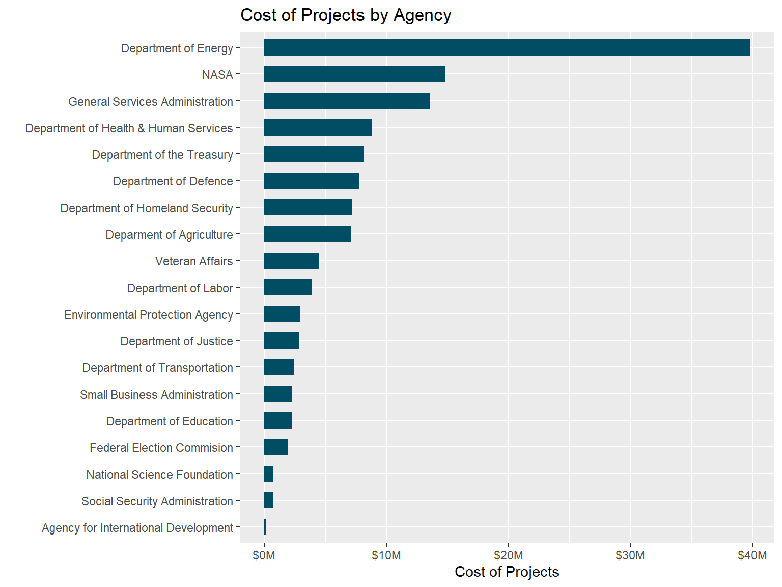
Costs by Agency

Code

#Visualizing the Costs

counts_by_agency |>
  select(agency, sum_w_gross) |>
  mutate(agency = fct_reorder(agency, sum_w_gross)) |>
  ggplot(aes(x = agency, y = sum_w_gross)) +
    geom_bar(stat = "identity", fill = '#014d64', width=.6) +
    scale_y_continuous(labels = label_number(prefix = "$", suffix = "M", scale = 1e-6, big.mark = ",")) +
    coord_flip() +
    theme(legend.title=element_blank()) +
    labs(title = "Cost of Projects by Agency",
        x = "",
        y = "Cost of Projects")

Summary Table by Agencies

Code

#Preparing Final Summary Table

counts_by_agency <- counts_by_agency |>
  left_join(counts_contrib, join_by(Agency == agency)) |>
  select(!index)


counts_by_agency <- counts_by_agency |>
  rename(Contributors = contributors)

counts_by_agency

--- title: "Code.gov" editor: markdown: wrap: 72 format: html: code-fold: true code-tools: true df-print: paged fig-width: 8 fig-height: 6 --- Code.gov is the Federal Government's platform for sharing and open sourcing software from Government Agencies. Recent policies of the U.S. Federal Government such as the Federal Source Code Policy (FSCP) promote the sharing of software source code developed by or for the Federal Government. Public funding for creation of software by or for the Federal Government and for research through universities plays an important role but it is not fully accounted. Our aim is to measure how much of OSS is developed in the U.S. Federal Government and estimate its value. As OSS is disseminated online, a wealth of information is available in the code and source code repositories of the software programs themselves. Examples include: contributors, their organizations, lines of code contributed, etc. We use non-survey data from Code.gov which is the Federal Government's platform for sharing and open sourcing software from Government Agencies. ## Objectives Our aim is to measure how much of OSS is developed in the U.S. Federal Government and estimate its value. This page below provides insights from Exploratory Data Analysis ## Data and Methods The data acquired from Code.gov is in JSON format covering over 17,000 software projects, across 21 different Federal Agencies and includes information on each project, agency name, host links, descriptions and other information. Most of these are developed and hosted on GitHub. We also use GitHub to obtain related information. Our second source of data is GitHub -- a popular version control and hosting service which is the largest platform in the world with over 108 million users and 100 million public repositories. From GitHub we have collected data on over 7.8 million repositories, 2.1 million users and 778 million commits. The information gathered from GitHub includes commits, lines of code added and deleted, OSI licenses, users' login information, organization, locations, emails, etc. ## Exploratory Data Analysis Add text here ```{r, include=FALSE} library(tidyverse) library(ggthemes) library(SnowballC) library(tidytext) library(igraph) library(ggraph) library(widyr) library(tidyorgs) library(treemap) library(treemapify) library(cranlogs) library(reticulate) library(RMySQL) library(DBI) library(RColorBrewer) library(kableExtra) library(knitr) library(corrplot) library(plotly) library(classInt) library(diverstidy) library(gridExtra) library(pander) library(dplyr) library(ggplot2) library(forcats) library(tidyr) library(treemap) library(treemapify) library(scales) Sys.setenv(DB_USERNAME = 'admin', DB_PASSWORD = 'OSS022323') ``` ### Hosting Platforms ```{r, message=FALSE} # establishing connection and listing all tables in database con <- dbConnect(MySQL(), user = Sys.getenv("DB_USERNAME"), password = Sys.getenv("DB_PASSWORD"), dbname = "codegov", host = "oss-1.cij9gk1eehyr.us-east-1.rds.amazonaws.com") hosting <- dbReadTable(con, "codegov_agency_hosting") dbDisconnect(con) hosting <- hosting |> mutate(total_hosting = rowSums(across(where(is.numeric)))) |> select(domain, total_hosting) |> filter(!row_number() %in% c(10)) #theme_set(theme_wes()) hosting |> mutate(domain = fct_reorder(domain, total_hosting)) |> ggplot(aes(x = domain, y = total_hosting)) + geom_bar(stat = "identity", fill = '#014d64', width=.6) + coord_flip() + theme(legend.title=element_blank()) + labs(title = "Hosting Platforms by Projects Hosted", subtitle = "Github is the most popular hosting platform", x = "Hosting Platform", y = "Count of Projects") ``` The most popular hosting platform for Code.gov projects is GitHub followed by the Code.gov platform itself. ### Government Agencies ```{r} # establishing connection and listing all tables in database con <- dbConnect(MySQL(), user = Sys.getenv("DB_USERNAME"), password = Sys.getenv("DB_PASSWORD"), dbname = "codegov", host = "oss-1.cij9gk1eehyr.us-east-1.rds.amazonaws.com") agency <- dbReadTable(con, "codegov_gh_agency_count") dbDisconnect(con) agency |> select(agency, projects) |> mutate(agency = fct_reorder(agency, projects)) |> ggplot(aes(x = agency, y = projects)) + geom_bar(stat = "identity", fill = '#014d64', width=.6) + coord_flip() + theme(legend.title=element_blank()) + labs(title = "Number of Projects by Agency", x = "", y = "Count of Projects") ``` The Department of Energy, the General Services Administration and the Department of Health & Human Services are the top 3 agencies by number of projects showcased on the Code.gov platform. ### Contributing Sectors ```{r, message=FALSE} # establishing connection and listing all tables in database con <- dbConnect(MySQL(), user = Sys.getenv("DB_USERNAME"), password = Sys.getenv("DB_PASSWORD"), dbname = "codegov", host = "oss-1.cij9gk1eehyr.us-east-1.rds.amazonaws.com") sectors <- dbReadTable(con, "codegov_users_sectored") dbDisconnect(con) sectors_count <- sectors |> summarise(Academic = sum(academic, na.rm = T), Business = sum(business, na.rm = T), Government = sum(government, na.rm = T), `Non-Profit` = sum(nonprofit, na.rm = T)) sectors_count <- sectors_count |> gather(key = "Sectors", value = "Contributors") ggplot(sectors_count, aes(area = Contributors, fill = Sectors, label = Contributors)) + geom_treemap() + geom_treemap_text(colour = "black", place = "centre", size = 15)+ ggtitle("Number of Contributors Per Sector")+ scale_fill_economist() ``` Contributors belonging to the Government sector were the highest with 6,324 contributors followed by the Academic sector with 2,635 contributors, Business sector with 1,615 contributors and the Non-Profit sector with 232 contributors. ### Top 20 Organizations By Number of Contributors ```{r} # establishing connection and listing all tables in database con <- dbConnect(MySQL(), user = Sys.getenv("DB_USERNAME"), password = Sys.getenv("DB_PASSWORD"), dbname = "codegov", host = "oss-1.cij9gk1eehyr.us-east-1.rds.amazonaws.com") users <- dbReadTable(con, "codegov_users_sectors") dbDisconnect(con) orgs_count <- users |> count(organization, name = 'Contributors', sort = T) |> rename(Organization = organization) |> arrange(desc(Contributors)) |> top_n(21, Contributors) |> slice(2:21) orgs_count |> select(Organization, Contributors) |> mutate(Organization = fct_reorder(Organization, Contributors)) |> ggplot(aes(x = Organization, y = Contributors)) + geom_bar(stat = "identity", fill = '#014d64', width=.6) + coord_flip() + geom_text(aes(label=Contributors), color='white', position=position_dodge(width = 0.05), hjust=1.2, size = 7/.pt) + theme(legend.title=element_blank()) + labs(title = "Number of Contributors by Organization", x = "", y = "Count of Contributors") ``` The highest number of contributors by organizations were the Lawrence Livermore National Laboratory and Sandia National Laboratory. Private sector organizations with the highest number of contributors were Intel Corporation and Google. ### Top 20 Contributors by Lines of Code Added ```{r, warning=FALSE} #establishing connection and listing all tables in database con <- dbConnect(MySQL(), user = Sys.getenv("DB_USERNAME"), password = Sys.getenv("DB_PASSWORD"), dbname = "codegov", host = "oss-1.cij9gk1eehyr.us-east-1.rds.amazonaws.com") contri <- dbReadTable(con, "codegov_gh_commits_by_login") dbDisconnect(con) cont_count <- contri |> select(login, additions) |> group_by(login) |> summarise(Contribution = sum(additions)) |> rename(Contributor = login) |> arrange(desc(Contribution)) |> top_n(20, Contribution) cont_count |> select(Contributor, Contribution) |> mutate(Contributor = fct_reorder(Contributor, Contribution)) |> ggplot(aes(x = Contributor, y = Contribution)) + geom_bar(stat = "identity", fill = '#014d64', width=.6) + scale_y_continuous(labels = label_number(suffix = "M", scale = 1e-6, big.mark = ",")) + coord_flip() + theme(legend.title=element_blank()) + labs(title = "Lines of Code Contributed by Top 20 Contributors", x = "", y = "Lines of Code") ``` ### Detailed Info of Top 20 Contributors (Table) ```{r} top_20_users <- cont_count %>% left_join(users, by = join_by(Contributor == login)) |> group_by(Contributor) |> filter(row_number()==1) top_20_users ``` ### Top 20 Academic Institutions By Number of Contributors ```{r} # establishing connection and listing all tables in database con <- dbConnect(MySQL(), user = Sys.getenv("DB_USERNAME"), password = Sys.getenv("DB_PASSWORD"), dbname = "codegov", host = "oss-1.cij9gk1eehyr.us-east-1.rds.amazonaws.com") users <- dbReadTable(con, "codegov_users_sectors") dbDisconnect(con) orgs_count <- users |> filter(sector == 'Academic') |> count(organization, name = 'Contributors', sort = T) |> rename(Organization = organization) |> arrange(desc(Contributors)) |> top_n(20, Contributors) orgs_count |> select(Organization, Contributors) |> mutate(Organization = fct_reorder(Organization, Contributors)) |> ggplot(aes(x = Organization, y = Contributors)) + geom_bar(stat = "identity", fill = '#014d64', width=.6) + coord_flip() + geom_text(aes(label=Contributors), color='white', position=position_dodge(width = 0.05), hjust=1.2, size = 7/.pt) + theme(legend.title=element_blank()) + labs(title = "Top 20 Academic Insitutions by Contributors", x = "", y = "Count of Contributors") ``` Stanford University is the academic institution with the highest number of contributors followed by University of California - Berkeley and University of Michigan - Ann Arbor. ### Top 20 Contributing Research Labs ```{r} # establishing connection and listing all tables in database con <- dbConnect(MySQL(), user = Sys.getenv("DB_USERNAME"), password = Sys.getenv("DB_PASSWORD"), dbname = "codegov", host = "oss-1.cij9gk1eehyr.us-east-1.rds.amazonaws.com") users <- dbReadTable(con, "codegov_users_sectors") dbDisconnect(con) orgs_count <- users |> filter(grepl('Laboratory', organization)) |> count(organization, name = 'Contributors', sort = T) |> rename(Organization = organization) |> arrange(desc(Contributors)) |> top_n(20, Contributors) orgs_count |> select(Organization, Contributors) |> mutate(Organization = fct_reorder(Organization, Contributors)) |> ggplot(aes(x = Organization, y = Contributors)) + geom_bar(stat = "identity", fill = '#014d64', width=.6) + geom_text(aes(label=Contributors), color='#014d64', position=position_dodge(width=0.5), hjust=-0, size = 9/.pt) + coord_flip() + theme(legend.title=element_blank()) + labs(title = "Top 20 Labs by Contributors", x = "", y = "Count of Contributors") ``` The Lawrence Livermore National Laboratory is has the highest number of contributors out of all Laboratories. ### Top 20 Contributing Businesses ```{r} # establishing connection and listing all tables in database con <- dbConnect(MySQL(), user = Sys.getenv("DB_USERNAME"), password = Sys.getenv("DB_PASSWORD"), dbname = "codegov", host = "oss-1.cij9gk1eehyr.us-east-1.rds.amazonaws.com") users <- dbReadTable(con, "codegov_users_sectors") dbDisconnect(con) orgs_count <- users |> filter(sector == 'Business') |> count(organization, name = 'Contributors', sort = T) |> rename(Organization = organization) |> arrange(desc(Contributors)) |> top_n(20, Contributors) orgs_count |> select(Organization, Contributors) |> mutate(Organization = fct_reorder(Organization, Contributors)) |> ggplot(aes(x = Organization, y = Contributors)) + geom_bar(stat = "identity", fill = '#014d64', width=.6) + coord_flip() + geom_text(aes(label=Contributors), color='white', position=position_dodge(width = 0.05), hjust=1.2, size = 7/.pt) + theme(legend.title=element_blank()) + labs(title = "Top 20 Businesses by Contributors", x = "", y = "Count of Contributors") ``` Intel Corporation, Google and Kitware are the top 3 corporations with the highest number of contributors. ------------------------------------------------------------------------ ## Cost Calculations ```{r, message=FALSE, warning=FALSE} # establishing connection and listing all tables in database con <- dbConnect(MySQL(), user = Sys.getenv("DB_USERNAME"), password = Sys.getenv("DB_PASSWORD"), dbname = "codegov", host = "oss-1.cij9gk1eehyr.us-east-1.rds.amazonaws.com") counts_repo <- dbReadTable(con, "codegov_gh_commits_by_agency") dbDisconnect(con) ``` ```{r, include=FALSE} #Aggregating the lines of code by Agency counts_agency <- counts_repo |> group_by(agency) |> summarise(total_commits = sum(commits), total_additions = sum(additions), total_deletions = sum(deletions), total_sum_adds_dels = sum(sum_adds_dels), total_net_adds_dels = sum(net_adds_dels) ) ``` ```{r, include=FALSE} #Renaming the Agencies row_values <- c("Department of Defence", "Department of Energy", "Department of Homeland Security", "Department of Justice", "Department of Labor", "Department of Education", "Federal Election Commision", "Environmental Protection Agency", "General Services Administration", "Department of Health & Human Services", "Agency for International Development", "NASA", "National Science Foundation", "Social Security Administration", "Small Business Administration", "Department of Transportation", "Department of the Treasury", "Deparment of Agriculture", "Veteran Affairs") counts_agency <- counts_agency |> mutate(agency = row_values) ``` ```{r, include=FALSE} #Calculating the Costs library(data.table) counts_by_agency <- as.data.table(counts_agency) #COST BASED ON Additions counts_by_agency[,adds_wo_gross := round(22094.19 * 2.5 * (2.4 * (total_additions/1000)^1.05)^0.38,2)] counts_by_agency[,adds_w_gross := round(27797.24 * 2.5 * (2.4 * (total_additions/1000)^1.05)^0.38,2)] #COST BASED ON Additions + Deletions counts_by_agency[,sum_wo_gross := round(22094.19 * 2.5 * (2.4 * (total_sum_adds_dels/1000)^1.05)^0.38,2)] counts_by_agency[,sum_w_gross := round(27797.24 * 2.5 * (2.4 * (total_sum_adds_dels/1000)^1.05)^0.38,2)] #COST BASED ON Additions - Deletions counts_by_agency[,net_wo_gross := round(22094.19 * 2.5 * (2.4 * (total_net_adds_dels/1000)^1.05)^0.38,2)] counts_by_agency[,net_w_gross := round(27797.24 * 2.5 * (2.4 * (total_net_adds_dels/1000)^1.05)^0.38,2)] counts_by_agency %>% count() # 7751144 repos counts_by_agency %>% distinct(agency) %>% count() # 7751144 ``` #### Costs by Agency ```{r} #Visualizing the Costs counts_by_agency |> select(agency, sum_w_gross) |> mutate(agency = fct_reorder(agency, sum_w_gross)) |> ggplot(aes(x = agency, y = sum_w_gross)) + geom_bar(stat = "identity", fill = '#014d64', width=.6) + scale_y_continuous(labels = label_number(prefix = "$", suffix = "M", scale = 1e-6, big.mark = ",")) + coord_flip() + theme(legend.title=element_blank()) + labs(title = "Cost of Projects by Agency", x = "", y = "Cost of Projects") ``` ```{r, include=FALSE} #Creating Summary Table counts_by_agency <- counts_by_agency |> select(agency, total_commits, total_additions, adds_w_gross) |> left_join(agency, join_by(agency)) |> rename(Agency = agency, Commits = total_commits, `Lines of Code` = total_additions, `Cost of Development` = adds_w_gross, Projects = projects, ) counts_by_agency$Agency[counts_by_agency$Agency == 'NASA'] <- 'National Aeronautics and Space Administration' ``` ```{r, include=FALSE,message=FALSE, warning=FALSE} # establishing connection and listing all tables in database con <- dbConnect(MySQL(), user = Sys.getenv("DB_USERNAME"), password = Sys.getenv("DB_PASSWORD"), dbname = "codegov", host = "oss-1.cij9gk1eehyr.us-east-1.rds.amazonaws.com") counts_contrib <- dbReadTable(con, "codegov_agency_contributors") dbDisconnect(con) ``` #### Summary Table by Agencies ```{r} #Preparing Final Summary Table counts_by_agency <- counts_by_agency |> left_join(counts_contrib, join_by(Agency == agency)) |> select(!index) counts_by_agency <- counts_by_agency |> rename(Contributors = contributors) counts_by_agency ```