R (CRAN)

Data Preparation and Cleaning

In this section, we go over the how the data was collected, a general of what the data contains, including things like the number of packages obtained and any missing data, and the cleaning processes that were done to make the data fit for the analysis. The data was collected through a function R provides to connect to the CRAN database to obtain metadata on all packages that currently exist. Total downloads is not included already when the CRAN database is loaded, so another R function from the Cranlogs package is used to obtain this information for each individual package (We explain this process in another R script and upload the result to our database). The cleaning and analysis processes included selecting only the variables we were interested in for further analysis for specific packages (Package Name, Authors, Maintainers, Titles of packages, Descriptions of packages, Dependencies, Reverse_Dependencies, All-time download counts and Normalized download counts, and Github URLs), cleaning text data for character variables like dependencies and author names, and extracting institution and sector information from maintainer emails. After the initial data preparation and cleaning processes, we present a few figures from the exploratory data analysis.

Listing and Selecting Variables from CRAN Database

This function loads the CRAN database for all package metadata. We also load in the package download by year data and join it to the CRAN database after calculating all-time downloads and normalized downloads (Downloads/Number of years of Downloaod data available for).

Code

#### loading downloads
Cran_Downloads_Year <- dbReadTable(con, "package_downloads")

# load in R CRAN database
cran <- tools::CRAN_package_db()

# Filtering for unique package names

cran <- cran %>%
           distinct(Package, .keep_all = T)

## Create Downloads all-time and Downloads normalized
Cran_Downloads_Year <- Cran_Downloads_Year %>%
  group_by(Package) %>%
  mutate(
    Downloads_All_Time = sum(Downloads),
    Downloads_Normalized = round(sum(Downloads) / n())
  ) %>%
  ungroup()

## Join Download Data to df

Download_Data <- Cran_Downloads_Year %>%
  select(Package, Downloads_All_Time, Downloads_Normalized) %>%
  distinct(Package, .keep_all = TRUE)

cran <- cran %>% left_join(Download_Data, by = "Package")


colnames(cran)[63] <- "Reverse_Depends"

There are 69 columns of metadata available for each package (Including the derived download variables), but as stated in the introduction, we are only interested in a select amount. We still output a table with all variables and a short description for each.

Code

# Create a dataframe
variables <- c("Package", "Version", "Priority", "Depends", "Imports", "LinkingTo", 
               "Suggests", "Enhances", "License", "License_is_FOSS", "License_restricts_use", 
               "OS_type", "Archs", "MD5sum", "NeedsCompilation", "Additional_repositories", 
               "Author", "Authors@R", "Biarch", "BugReports", "BuildKeepEmpty", "BuildManual", 
               "BuildResaveData", "BuildVignettes", "Built", "ByteCompile", "Classification/ACM", 
               "Classification/ACM-2012", "Classification/JEL", "Classification/MSC", 
               "Classification/MSC-2010", "Collate", "Collate.unix", "Collate.windows", "Contact", 
               "Copyright", "Date", "Date/Publication", "Description", "Encoding", "KeepSource", 
               "Language", "LazyData", "LazyDataCompression", "LazyLoad", "MailingList", "Maintainer", 
               "Note", "Packaged", "RdMacros", "StagedInstall", "SysDataCompression", 
               "SystemRequirements", "Title", "Type", "URL", "UseLTO", "VignetteBuilder", "ZipData", 
               "Path", "X-CRAN-Comment", "Published", "Reverse depends", "Reverse imports", 
               "Reverse linking to", "Reverse suggests", "Reverse enhances", "Downloads_All_Time",
               "Downloads_Normalized")

descriptions <- c("The name of the package.", "The version of the package.", 
                  "If the package is a base or recommended package.", 
                  "A list of packages that this package depends on.", 
                  "A list of packages this package imports.", 
                  "A list of packages this package is linking to at the C/C++ level.", 
                  "A list of packages this package suggests for additional functionality.", 
                  "A list of packages this package enhances, but does not depend on.", 
                  "The license of the package.", 
                  "Whether the license is free and open-source.", 
                  "Whether the license restricts use.", 
                  "Operating system type.", "Architecture the package is built for.", 
                  "The MD5 checksum of the package file.", 
                  "Whether the package needs compilation.", 
                  "Any additional repositories where this package can be found.", 
                  "The author(s) of the package.", 
                  "The author(s) of the package in machine-readable form.", 
                  "Whether the package can be installed on both 32 and 64-bit systems.", 
                  "The URL for reporting bugs.", 
                  "Whether to keep empty directories when building the package.", 
                  "Whether to build the package manual.", 
                  "Whether to resave the data when building the package.", 
                  "Whether to build vignettes when building the package.", 
                  "The R version the package was built under.", 
                  "Whether to byte-compile the package.", 
                  "The ACM classification of the package.", 
                  "The ACM-2012 classification of the package.", 
                  "The JEL classification of the package.", 
                  "The MSC classification of the package.", 
                  "The MSC-2010 classification of the package.", 
                  "The collation order for the package documentation.", 
                  "The Unix-specific collation order for the package documentation.", 
                  "The Windows-specific collation order for the package documentation.", 
                  "The contact information for the package maintainer.", 
                  "The copyright notice for the package.", 
                  "The date the package was published.", 
                  "The date the package was published.", 
                  "A description of the package.", 
                  "The character encoding of the package files.", 
                  "Whether to keep the source code when building the package.", 
                  "The language(s) the package is available in.", 
                  "Whether the data in the package is loaded lazily.", 
                  "The compression type for lazy data loading.", 
                  "Whether the package uses lazy loading.", 
                  "The URL for the package mailing list.", 
                  "The package maintainer.", "Any additional notes about the package.", 
                  "The date the package was packaged.", 
                  "Whether the package uses Rd macros.", 
                  "Whether the package uses staged installation.", 
                  "The type of system data compression used.", 
                  "Any system requirements for the package.", 
                  "The title of the package.", 
                  "The type of package (e.g., 'Package', 'Data', 'Documentation', etc.).", 
                  "The URL for the package, if available.", 
                  "Whether the package uses Link-Time Optimization.", 
                  "The package(s) used to build the vignettes.", 
                  "Whether the data directory should be zipped.", 
                  "The path of the package directory.", 
                  "Any additional comments from CRAN.", 
                  "Whether the package is published.", 
                  "Other packages that depends on this package.", 
                  "Other packages that imports this package.", 
                  "Other packages that link to this package.", 
                  "Other packages that suggests this package.", 
                  "Other packages that enhances this package.",
                  "Number of all-time downloads for this package",
                  "All-time downloads divided by number of years the package has exsited.")

Variable_df <- data.frame(variables, descriptions)


Variable_df %>%
  kbl(caption = "Variable Descriptions for CRAN Database", escape = F, 
      col.names = c("Variables", "Descriptions"))%>%
  kable_classic()%>%
  kable_styling(font_size = 12,  full_width = T)%>%
 row_spec(0, bold = T, background = , color = "white")%>%
   column_spec(1, bold = T, border_right = T)%>%
  scroll_box(width = "100%", height = "500px") 

Variable Descriptions for CRAN Database

Variables	Descriptions
Package	The name of the package.
Version	The version of the package.
Priority	If the package is a base or recommended package.
Depends	A list of packages that this package depends on.
Imports	A list of packages this package imports.
LinkingTo	A list of packages this package is linking to at the C/C++ level.
Suggests	A list of packages this package suggests for additional functionality.
Enhances	A list of packages this package enhances, but does not depend on.
License	The license of the package.
License_is_FOSS	Whether the license is free and open-source.
License_restricts_use	Whether the license restricts use.
OS_type	Operating system type.
Archs	Architecture the package is built for.
MD5sum	The MD5 checksum of the package file.
NeedsCompilation	Whether the package needs compilation.
Additional_repositories	Any additional repositories where this package can be found.
Author	The author(s) of the package.
Authors@R	The author(s) of the package in machine-readable form.
Biarch	Whether the package can be installed on both 32 and 64-bit systems.
BugReports	The URL for reporting bugs.
BuildKeepEmpty	Whether to keep empty directories when building the package.
BuildManual	Whether to build the package manual.
BuildResaveData	Whether to resave the data when building the package.
BuildVignettes	Whether to build vignettes when building the package.
Built	The R version the package was built under.
ByteCompile	Whether to byte-compile the package.
Classification/ACM	The ACM classification of the package.
Classification/ACM-2012	The ACM-2012 classification of the package.
Classification/JEL	The JEL classification of the package.
Classification/MSC	The MSC classification of the package.
Classification/MSC-2010	The MSC-2010 classification of the package.
Collate	The collation order for the package documentation.
Collate.unix	The Unix-specific collation order for the package documentation.
Collate.windows	The Windows-specific collation order for the package documentation.
Contact	The contact information for the package maintainer.
Copyright	The copyright notice for the package.
Date	The date the package was published.
Date/Publication	The date the package was published.
Description	A description of the package.
Encoding	The character encoding of the package files.
KeepSource	Whether to keep the source code when building the package.
Language	The language(s) the package is available in.
LazyData	Whether the data in the package is loaded lazily.
LazyDataCompression	The compression type for lazy data loading.
LazyLoad	Whether the package uses lazy loading.
MailingList	The URL for the package mailing list.
Maintainer	The package maintainer.
Note	Any additional notes about the package.
Packaged	The date the package was packaged.
RdMacros	Whether the package uses Rd macros.
StagedInstall	Whether the package uses staged installation.
SysDataCompression	The type of system data compression used.
SystemRequirements	Any system requirements for the package.
Title	The title of the package.
Type	The type of package (e.g., 'Package', 'Data', 'Documentation', etc.).
URL	The URL for the package, if available.
UseLTO	Whether the package uses Link-Time Optimization.
VignetteBuilder	The package(s) used to build the vignettes.
ZipData	Whether the data directory should be zipped.
Path	The path of the package directory.
X-CRAN-Comment	Any additional comments from CRAN.
Published	Whether the package is published.
Reverse depends	Other packages that depends on this package.
Reverse imports	Other packages that imports this package.
Reverse linking to	Other packages that link to this package.
Reverse suggests	Other packages that suggests this package.
Reverse enhances	Other packages that enhances this package.
Downloads_All_Time	Number of all-time downloads for this package
Downloads_Normalized	All-time downloads divided by number of years the package has exsited.

After selecting only the variables of interest and filtering for unique names in the package field, we find that there are 19852 packages currently on CRAN (9/7/2023).

Code

# selecting variables of interest
cran <- cran %>%
 select(Package, Depends, License, Author, 
          Description, Maintainer, Title, URL, Reverse_Depends, Downloads_Normalized, Downloads_All_Time) 

Missing Data

When taking a look at missing data, all packages have available information for Titles, Descriptions, Authors, Maintainers, and URLs. There are about 26% of packages that do not have any dependencies listed, and 92% of packages do not have reverse dependencies, but this is expected, as some packages do not have dependencies or reverse dependencies in their metadata based on the CRAN URLs. Therefore, we do not list this as missing data in the table. Furthermore, about 45% of the packages do not have a URL pointing to another homepage other than the standard CRAN URL.

Code

##### Looking at missing data ######

## How many packages have.... ##

## Titles
cran %>% 
    summarise(Title = mean(!is.na(Title)))

## Description
cran %>% 
    summarise(Description = mean(!is.na(Description)))

## Dependencies
cran %>% 
    summarise(Dependencies = mean(!is.na(Depends)))

## Authors
cran %>% 
    summarise(Author = mean(!is.na(Author)))

## Maintainer
cran %>% 
    summarise(Maintainer = mean(!is.na(Maintainer)))

## URL
cran %>% 
    summarise(URL = mean(!is.na(URL)))


## Reverse Depends
cran %>% 
    summarise(Reverse_Depends = mean(!is.na(Reverse_Depends)))

Code

### Creating missing table

Variable <- c( "Title", "Description", "Author","Depends", "Reverse Depends",
"Maintainer", "URL")

Missing <- c("0%", "0%", "0%", "0%", "0%", "0%", "45%")

Cran_missing <- as.data.frame(cbind(Variable, Missing))

Cran_missing %>%
  kbl(caption = "Missing Data for CRAN Packages", escape = F)%>%
  kable_classic()%>%
   kable_styling(font_size = 12, full_width = T)%>%
 row_spec(0, bold = T, background = '#014d64', color = "white")

Missing Data for CRAN Packages

Variable	Missing
Title	0%
Description	0%
Author	0%
Depends	0%
Reverse Depends	0%
Maintainer	0%
URL	45%

Cleaning Text Data

This code chunk removes the brackets and other text within the authors field that is not needed for counting the number of authors per package. This wraps up the data collection, description, and cleaning processes that were done before beginning analysis. All other transformations and cleaning codes were used during the analysis process.

Code

###### Cleaning author data #####


## remove text between brackets

author_clean1 <- function(x){
  gsub("\\[[^]]*]", "",x)
}


## remove line breaks

author_clean2 <- function(x){
  gsub("[\r\n]", "", x)
}


### apply function to authors variables

cran$Author <- author_clean1(cran$Author)

cran$Author <- author_clean2(cran$Author)

Exploratory Data Analysis (EDA) of All R Packages on CRAN

This section contains an initial exploratory data analysis on the CRAN database, including the number of dependencies per package, the number of authors per package, number of reverse dependencies per package, and the download data for some of the top packages.

Count Data for Dependencies, Authors, and Reverse Dependencies

Here, we count the number of authors,dependencies, and reverse dependencies per packages, which are separated by commas, and then store it in an object called “Count_Data”. We join this data back to our original dataframe, “cran

Code

# Writing loop to count number of authors and dependencies across packages
Count_Data <- seq_len(nrow(cran)) %>%
  map_df(~{
    cran[.x, ] %>%
      select(Package, Depends, Author, Reverse_Depends) %>%
      map_df(~ifelse(is.na(.x), 0, length(str_split(.x, ",")[[1]]))) %>% ### Count objects separated by commas 
      mutate(Package = cran$Package[.x])
  }) %>%
  select(Package, Author, Depends, Reverse_Depends)

colnames(Count_Data) <- c("Package", "Author_Count", "Depends_Count", 
                          "Reverse_Depends_Count")

### Join the count variables
cran <- cran %>% left_join(Count_Data, by = "Package")

# Modify the author count to detect those with "and" and no commas as 2 authors, and count changed observations changed
cran <- cran %>%
  # Step 1: Create a new variable to record the previous Author_Count
  mutate(Previous_Author_Count = Author_Count) %>%
  # Step 2: Modify the Author_Count
  mutate(Author_Count = ifelse(str_detect(Author, "\\band\\b") & !str_detect(Author, ","), 2, Author_Count)) %>%
  # Step 3: Create a new variable to indicate if the Author_Count was changed
  mutate(Changed = ifelse(Author_Count != Previous_Author_Count, 1, 0))

Dependencies per Package

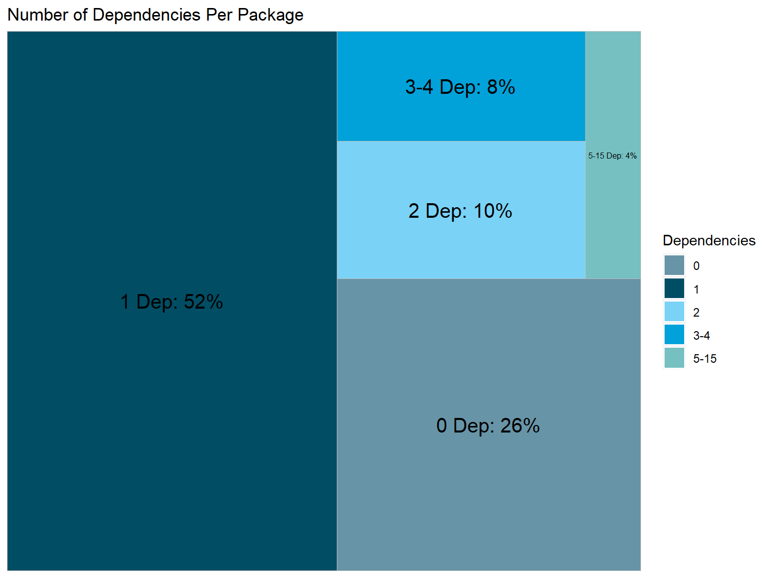
We will visualize the dependencies counts by creating numeric ranges and storing it in a factor variable. The factor categories are calculated using the “jenks” method, which tries to minimize the variance within factor categories and maximize the variance between factor categories. We output the table to construct percentage counts per category.

Code

### Creating categories for dependency counts

cran <- cran %>%
          mutate(Depends_Cat = case_when(Depends_Count == 0 ~ "0",
                                         Depends_Count  == 1 ~ "1",
                                         Depends_Count  == 2 ~ "2",
                                         Depends_Count  == 3 | Depends_Count == 4 ~ "3-4",
                                         Depends_Count  > 4 ~ "5-15"))
## converting to factor
cran$Depends_Cat <- as.factor(cran$Depends_Cat)

# Getting counts per category 
table(cran$Depends_Cat)

    0     1     2   3-4  5-15 
 5233 10402  1995  1625   702 

A little more than half of the packages 1 dependency, 26% have 0 dependencies listed, 10% have 2 dependencies, 8% have 3 to 4 dependencies, and 4% have 5 or more dependencies.

Code

### Creating inputs for tree map plot

Dependencies <- c("0", "1", "2", "3-4", "5-15")

Value <- c(26, 52, 10, 8, 4)

Label <- c("0 Dep: 26%", "1 Dep: 52%", "2 Dep: 10%", "3-4 Dep: 8%", "5-15 Dep: 4%")

Depends_Tree <- cbind(Dependencies, Value, Label)

Depends_Tree <- as.data.frame(Depends_Tree)

Depends_Tree$Value <- as.numeric(Depends_Tree$Value)

### Generating tree map plot

ggplot(Depends_Tree, aes(area = Value, fill = Dependencies, label = Label)) +
  geom_treemap() +
  geom_treemap_text(colour = "black",
                    place = "centre",
                    size = 15)+
  ggtitle("Number of Dependencies Per Package")+
  scale_fill_economist()

Authors per Package

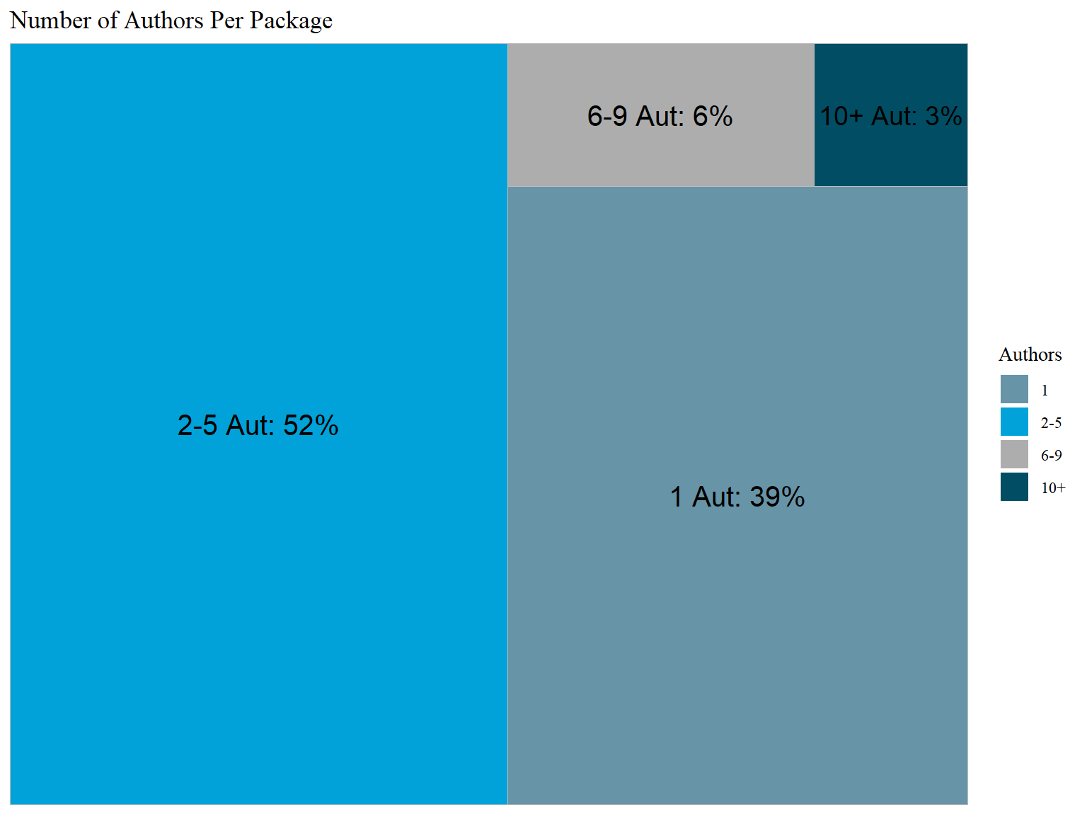
We know from looking at missing data that at least one author is present for each package. The author counts contain some extreme values some we take the log of authors to better show the distribution here.

Again, we do the same thing for authors that we did for dependencies, but instead of using the “jenks” method to determine breaks, we create factor categories based on single authors (1), smaller groups (2-5), medium sized groups (6-9), and large groups (10+). We are more concerned with the size of the group rather than trying to minimize variance within the separate groups for authors

Code

### Creating categories for numeric ranges 
cran <- cran %>%
         mutate(Authors_Cat = case_when(
                                         Author_Count == 1 ~ "1",
                                         Author_Count > 1 & Author_Count < 6 ~ "2-5",
                                         Author_Count > 5 & Author_Count < 10 ~ "6-9",
                                         Author_Count > 9  ~ "10+"))


### Assigning categorical variables to class factor and reordering
cran$Authors_Cat <- factor(cran$Authors_Cat, levels = c("1", "2-5", "6-9", "10+"))

### getting counts per category
table(cran$Authors_Cat)

    1   2-5   6-9   10+ 
 7768 10331  1323   535 

39% of packages have only one author, 52% have 2-5, 6% have 6-9, and only 3% have 10+ authors

Code

### Creating inputs for tree map plot

Authors <- c("1", "2-5", "6-9", "10+")

Value <- c(39, 52, 6, 3)

Label <- c("1 Aut: 39%", "2-5 Aut: 52%", "6-9 Aut: 6%", "10+ Aut: 3%")

Authors_Tree <- cbind(Authors, Value, Label)

Authors_Tree <- as.data.frame(Authors_Tree)

Authors_Tree$Value <- as.numeric(Authors_Tree$Value)


ggplot(Authors_Tree, aes(area = Value, fill = Authors, label = Label)) +
  geom_treemap() +
  geom_treemap_text(colour = "black",
                    place = "centre",
                    size = 15)+
  ggtitle("Number of Authors Per Package")+
  scale_fill_economist(breaks = c("1", "2-5", "6-9", "10+"))+ 
  theme_tufte()

Reverse Dependencies per Package

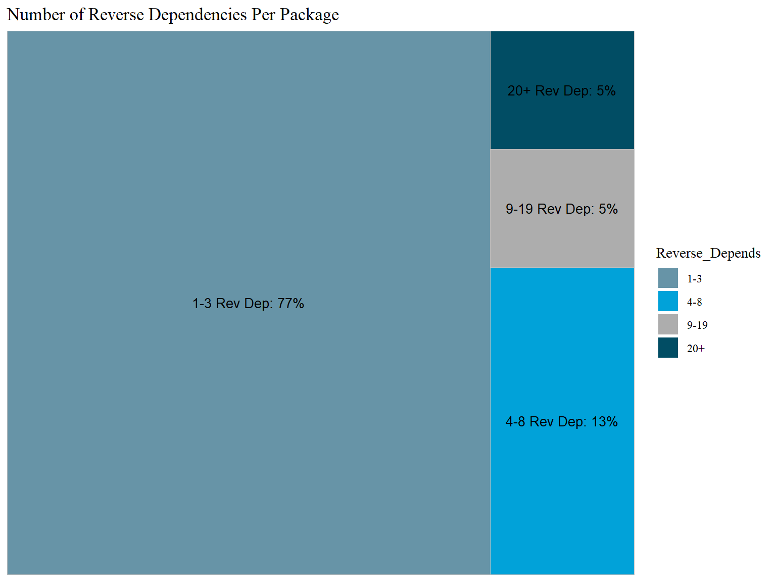
As we already know, most packages have 0 reverse dependencies (92%). We will subset to those that have at least one, and look further at that distribution in the histogram and TreeMap plot. After filtering for those with at least 1, we are left with 1644 total packages

Code

### Creating categories for numeric ranges 
cran <- cran %>%
         mutate(Reverse_Depends_Cat = case_when(
           
Reverse_Depends_Count > 0 & Reverse_Depends_Count < 4 ~ "1-3",

Reverse_Depends_Count > 3 & Reverse_Depends_Count < 9 ~ "4-8",
  
Reverse_Depends_Count > 8 & Reverse_Depends_Count < 20 ~ "9-19",

Reverse_Depends_Count > 19 ~ "20+",


))

### Assigning categorical variables to class factor
cran$Reverse_Depends_Cat <- as.factor(cran$Reverse_Depends_Cat)

### getting counts per category
table(cran$Reverse_Depends_Cat)

 1-3  20+  4-8 9-19 
1266   79  214   92 

Of the packages that have at least one reverse dependency, 77% have 1 to 3, 13% have 4 to 8, 5% have 9 to 19 and 5% have 20+. Recall that only 8% of the packages have any reverse dependencies to begin with.

Code

### Creating inputs for tree map plot

Reverse_Depends <- c("1-3", "4-8", "9-19", "20+")

Value <- c(77, 13, 5, 5)

Label <- c("1-3 Rev Dep: 77%", "4-8 Rev Dep: 13%", "9-19 Rev Dep: 5%", "20+ Rev Dep: 5%")

Reverse_Depends_Tree <- cbind(Reverse_Depends, Value, Label)

Reverse_Depends_Tree <- as.data.frame(Reverse_Depends_Tree)

Reverse_Depends_Tree$Value <- as.numeric(Reverse_Depends_Tree$Value)

ggplot(Reverse_Depends_Tree, aes(area = Value, fill = Reverse_Depends, label = Label)) +
  geom_treemap() +
  geom_treemap_text(colour = "black",
                    place = "centre",
                    size = 10)+
  ggtitle("Number of Reverse Dependencies Per Package")+
  scale_fill_economist(breaks = c("1-3", "4-8", "9-19", "20+"))+
  theme_tufte()

Identifying Organizations from Maintainer Emails

The organization is extracted from the maintainer email and then the tidyorgs package is used to categorize the email as belonging to either government, academic, nonprofit, or business. The data is saved in an object titled “Inst”. In the 19,852 packages, we were able to extract an organization from 6981 of them. If we filter by distinct emails only, there are 3830 observations total. The reason the same email can show up multiple times is because the same email can be a maintainer of multiple packages.

We will save institution, sector, and country analysis for our research question section in the analysis section. The purpose of this is to show how the data was collected before we move into that analysis

Code

##### Cleaning email variable to extract Organization ####

cran$email <- sub(".*<", "", cran$Maintainer)  
cran$email <- gsub(">", "", cran$email)


### posit is replaced with rstudio, as these are the same thing

cran$email  <- gsub("@posit.co", "@rstudio.com", cran$email)

# searching for government, academic, nonprofit, and business emails

user_emails_to_orgs1 <- cran %>%
  email_to_orgs(email, input = email, output = Institution, "government")

user_emails_to_orgs2 <- cran %>%
  email_to_orgs(email, input = email, output = Institution, "academic") 

user_emails_to_orgs3 <- cran %>%
  email_to_orgs(email, input = email, output = Institution, "nonprofit") 

user_emails_to_orgs4 <- cran %>%
  email_to_orgs(email, input = email, output = Institution, "business") 

# creating an identifier variable for type of institution

user_emails_to_orgs1$Sector <- "Government"

user_emails_to_orgs2$Sector <- "Academic"

user_emails_to_orgs3$Sector <- "Nonprofit"

user_emails_to_orgs4$Sector <- "Business"

# Binding to one dataframe

Inst <- as.data.frame(rbind(user_emails_to_orgs1, user_emails_to_orgs2, 
                            user_emails_to_orgs3, user_emails_to_orgs4))

# Filtering for distinct emails
Inst_filtered <- Inst %>%
                        distinct(email, .keep_all = T)

cran <- cran %>% left_join(Inst_filtered, by = "email")

### Create Mainatiner Name variable

cran$Maintainer_Name <- gsub(" <.*$", "", cran$Maintainer)

# Fill in those with the same Mainatinaer name to have the same institution
cran <- cran %>%
  group_by(Maintainer_Name) %>%
  fill(Sector, Institution, .direction = "downup") %>%
  ungroup()

Download Data

Number of Downloads

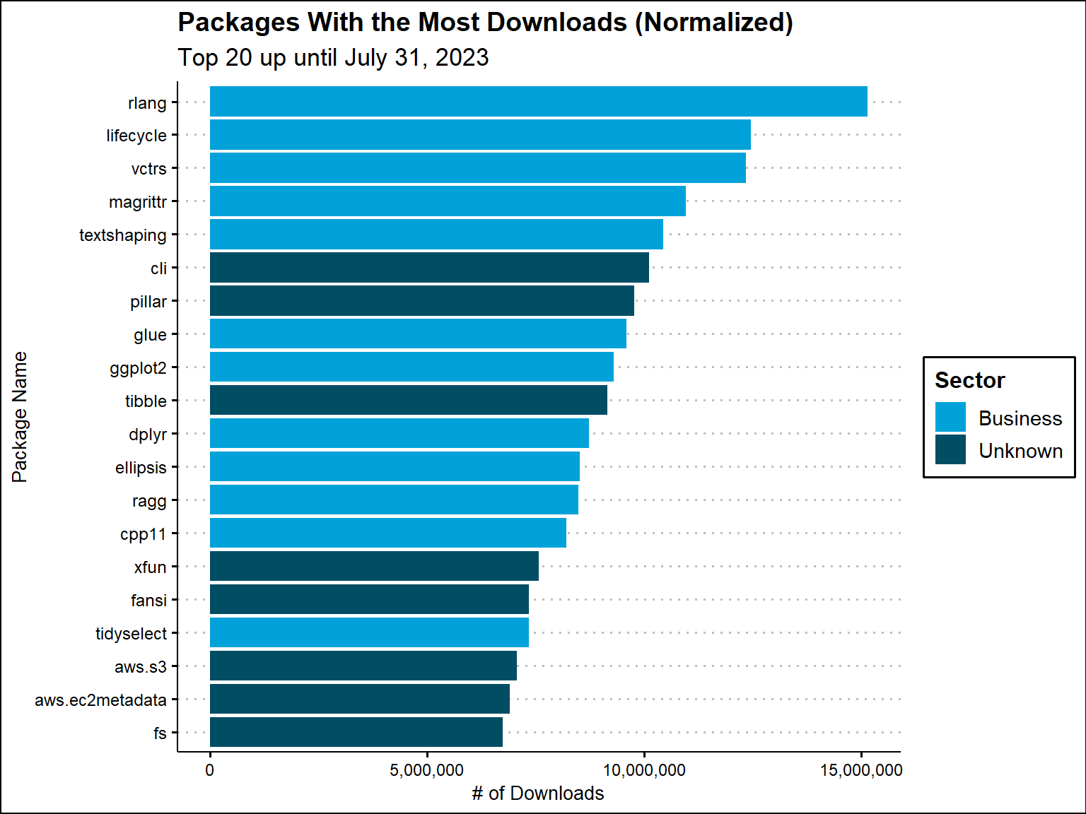
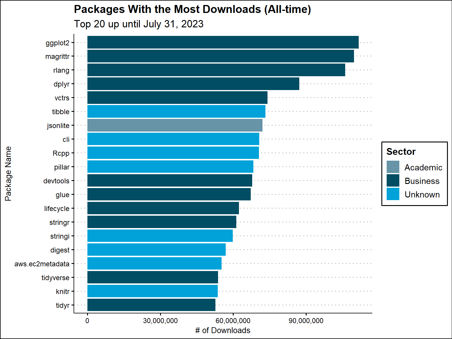
This shows the 20 packages with the most downloads all-time and normalized up to July 31st, 2023. GGplot2 is the number one package all-time, which makes sense, as data visualization is regarded as one of R’s major strong points. Magrittr has the second most and rlang has the third most. For normalized, the top 20 changes up slightly and rlang has the most based on normalized downloads. We also get an idea of the sectors for these packages.

Code

# replaces NAs with Unknown for graph output
cran$Sector[is.na(cran$Sector)] <- "Unknown"


all_possible_sectors <- c("Academic", "Business", "Nonprofit", "Government", "Unknown")

# Use the factor levels from the main 'cran' dataframe
cran$Sector <- factor(cran$Sector, levels = all_possible_sectors)

#-------------------------------------------------------------------------

### Getting the top 20 downloaded packages
 Top_20_Downloads_Normalized <-  cran %>%
  top_n(20, Downloads_Normalized)
  
  Top_20_Downloads_Normalized$Package <- factor(Top_20_Downloads_Normalized$Package, 
                           levels = Top_20_Downloads_Normalized$Package[order(Top_20_Downloads_Normalized$Downloads_Normalized)])
  
# Ensure that the Sector variable in your data frame has all these levels
Top_20_Downloads_Normalized$Sector <- factor(Top_20_Downloads_Normalized$Sector, levels = all_possible_sectors)
  
# plot the top 20
  Top_20_Downloads_Normalized %>%
ggplot(aes(x = Package, y = as.numeric(Downloads_Normalized), fill = Sector))+
    geom_bar(stat = "identity")+
    coord_flip()+
  ggtitle(label = "Packages With the Most Downloads (Normalized)",
          subtitle = "Top 20 up until July 31, 2023")+
  xlab("Package Name")+
  ylab("# of Downloads")+
    scale_y_continuous(labels = scales::comma)+
    scale_fill_economist()+
    theme_clean()
  
 #------------------------------------------------------------------------ 
  
### Getting the top 20 downloaded packages
 Top_20_Downloads_AT <-  cran %>%
  top_n(20, Downloads_All_Time)
  
  Top_20_Downloads_AT$Package <- factor(Top_20_Downloads_AT$Package, 
                           levels = Top_20_Downloads_AT$Package[order(Top_20_Downloads_AT$Downloads_All_Time)])
  
  
# Ensure that the Sector variable in your data frame has all these levels
Top_20_Downloads_AT$Sector <- factor(Top_20_Downloads_AT$Sector, levels = all_possible_sectors)
  
# plot the top 20
  Top_20_Downloads_AT %>%
ggplot(aes(x = Package, y = as.numeric(Downloads_All_Time), fill = Sector))+
    geom_bar(stat = "identity")+
    coord_flip()+
  ggtitle(label = "Packages With the Most Downloads (All-time)",
          subtitle = "Top 20 up until July 31, 2023")+
  xlab("Package Name")+
  ylab("# of Downloads")+
    scale_y_continuous(labels = scales::comma)+
    scale_fill_economist()+
    theme_clean()

Title Descriptions for Most Downloads

Here, we get some insight on what these top 20 packages are used for. It appears organization of data, visualizing data, and cleaning data are some of the key highlights from the top downloaded packages.

Code

Top_20_Downloads_Normalized %>%
  select(Package, Sector, Title, Downloads_Normalized)%>%
  arrange(desc(Downloads_Normalized))%>%
  kbl(caption = "Title Descriptions for the Most Downloaded Packages (Normalized)")%>%
  kable_classic()%>%
  kable_styling(font_size = 12,  full_width = T)%>%
 row_spec(0, bold = T, background = '#014d64', color = "white")%>%
  column_spec(1:3, border_right = T)%>%
  scroll_box()

Title Descriptions for the Most Downloaded Packages (Normalized)

Package	Sector	Title	Downloads_Normalized
rlang	Business	Functions for Base Types and Core R and 'Tidyverse' Features	15157282
lifecycle	Business	Manage the Life Cycle of your Package Functions	12466319
vctrs	Business	Vector Helpers	12354349
magrittr	Business	A Forward-Pipe Operator for R	10969342
textshaping	Business	Bindings to the 'HarfBuzz' and 'Fribidi' Libraries for Text Shaping	10439215
cli	Unknown	Helpers for Developing Command Line Interfaces	10113083
pillar	Unknown	Coloured Formatting for Columns	9766738
glue	Business	Interpreted String Literals	9597283
ggplot2	Business	Create Elegant Data Visualisations Using the Grammar of Graphics	9302718
tibble	Unknown	Simple Data Frames	9155589
dplyr	Business	A Grammar of Data Manipulation	8724160
ellipsis	Business	Tools for Working with ...	8513327
ragg	Business	Graphic Devices Based on AGG	8490946
cpp11	Business	A C++11 Interface for R's C Interface	8211148
xfun	Unknown	Supporting Functions for Packages Maintained by 'Yihui Xie'	7575899
fansi	Unknown	ANSI Control Sequence Aware String Functions	7345470
tidyselect	Business	Select from a Set of Strings	7343579
aws.s3	Unknown	'AWS S3' Client Package	7066464
aws.ec2metadata	Unknown	Get EC2 Instance Metadata	6898427
fs	Unknown	Cross-Platform File System Operations Based on 'libuv'	6751105

Code

Top_20_Downloads_AT %>%
  select(Package, Sector, Title, Downloads_All_Time)%>%
  arrange(desc(Downloads_All_Time))%>%
  kbl(caption = "Title Descriptions for the Most Downloaded Packages (All-time)")%>%
  kable_classic()%>%
  kable_styling(font_size = 12,  full_width = T)%>%
 row_spec(0, bold = T, background = '#014d64', color = "white")%>%
  column_spec(1:3, border_right = T)%>%
  scroll_box()

Title Descriptions for the Most Downloaded Packages (All-time)

Package	Sector	Title	Downloads_All_Time
ggplot2	Business	Create Elegant Data Visualisations Using the Grammar of Graphics	111632612
magrittr	Business	A Forward-Pipe Operator for R	109693420
rlang	Business	Functions for Base Types and Core R and 'Tidyverse' Features	106100971
dplyr	Business	A Grammar of Data Manipulation	87241601
vctrs	Business	Vector Helpers	74126095
tibble	Unknown	Simple Data Frames	73244712
jsonlite	Academic	A Simple and Robust JSON Parser and Generator for R	72078171
cli	Unknown	Helpers for Developing Command Line Interfaces	70791582
Rcpp	Unknown	Seamless R and C++ Integration	70645651
pillar	Unknown	Coloured Formatting for Columns	68367164
devtools	Business	Tools to Make Developing R Packages Easier	67790088
glue	Business	Interpreted String Literals	67180984
lifecycle	Business	Manage the Life Cycle of your Package Functions	62331594
stringr	Business	Simple, Consistent Wrappers for Common String Operations	61265559
stringi	Unknown	Fast and Portable Character String Processing Facilities	59874948
digest	Unknown	Create Compact Hash Digests of R Objects	56980817
aws.ec2metadata	Unknown	Get EC2 Instance Metadata	55187418
tidyverse	Business	Easily Install and Load the 'Tidyverse'	53736053
knitr	Unknown	A General-Purpose Package for Dynamic Report Generation in R	53724921
tidyr	Business	Tidy Messy Data	52663892

Saving dataframe for further analysis (Research Questions)

Code

cran <- cran %>%
  select(Package, URL, Maintainer, Maintainer_Name, email, Institution, Sector, Title, 
         Description, Depends, Depends_Count, Reverse_Depends, Reverse_Depends_Count, 
         Author, Author_Count, Downloads_All_Time, Downloads_Normalized)

### dbWriteTable(con, name = "package_database", cran)