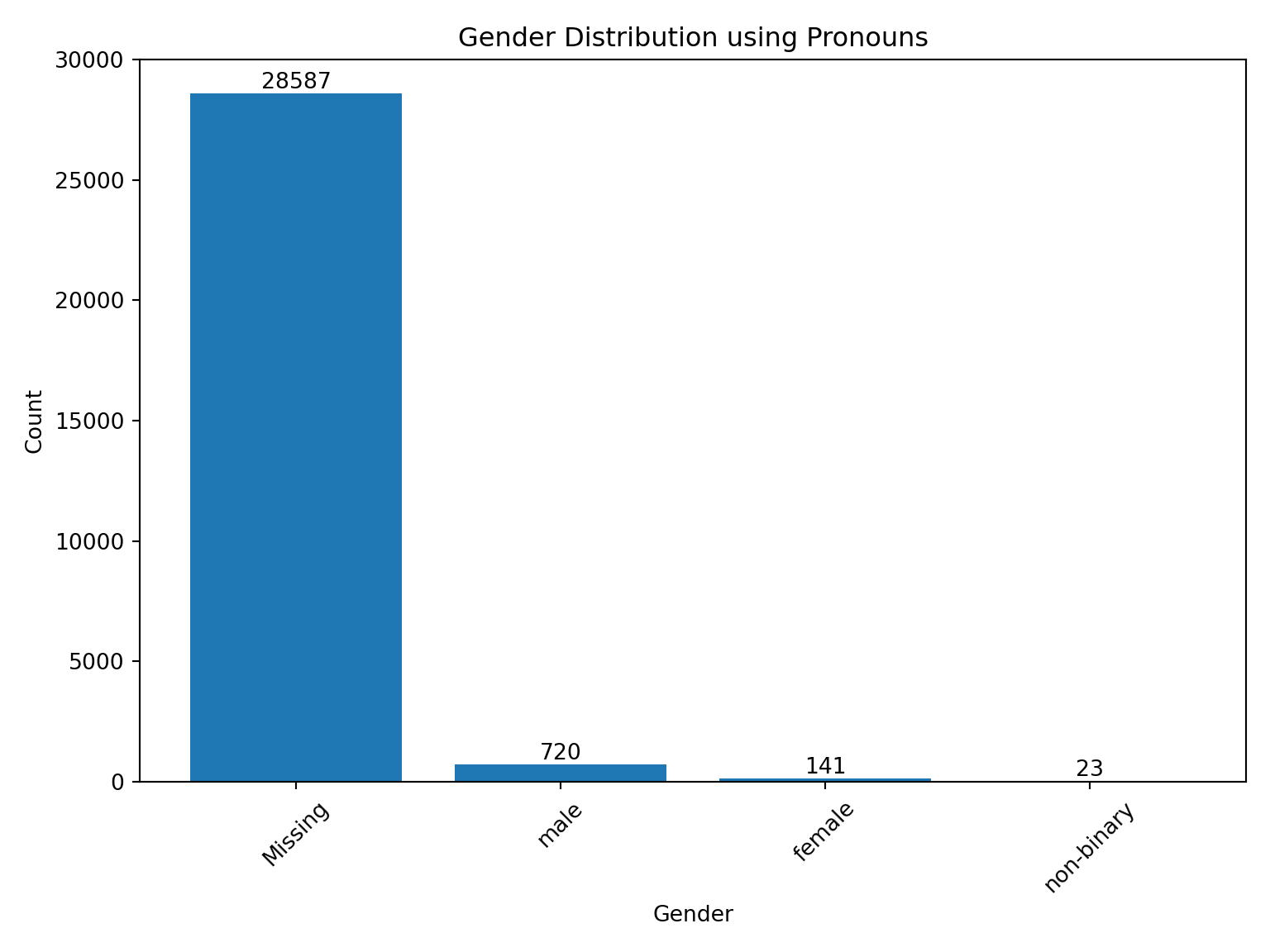
GitHub data contains pronouns for each user, we analyse this pronoun column and look for unique, blank and null values
Code
#| echo: falseimport pandas as pdimport numpy as npimport gender_guesser.detector as genderfrom sqlalchemy import create_engineimport pymysqlfrom sqlalchemy import texthostname="oss-1.cij9gk1eehyr.us-east-1.rds.amazonaws.com"dbname="cran"uname="jdpinto"pwd="DSPG2023"# Create SQLAlchemy engine to connect to MySQL Databaseengine = create_engine("mysql+pymysql://{user}:{pw}@{host}/{db}".format(host=hostname, db=dbname, user=uname, pw=pwd))query ='SELECT * FROM cran.cran_users'# Execute the query and load the results into a DataFrameuser = pd.read_sql(query, engine)def check_var(df,var): unique=df[var].nunique() blanks = df[df[var]==""].shape[0] nans = df[var].isna().sum()print("Unique values: ", unique, "\nBlanks: ", blanks, "\nNaNs: ", nans)print('For pronouns present in GitHub data: ')
For pronouns present in GitHub data:
Code
check_var(user, 'author_user_pronouns')
Unique values:  32
Blanks:  28586
NaNs:  0
While analyzing the pronoun data we found these pronouns entered by the users:
Code
invalid_cases=['Zurich, Switzerland','Chicago, IL, USA','Denver, CO','Wellington, New Zealand','Omaha, NE','Durham, UK','Barcelona','Flagstaff, AZ','Bamberg, Germany','Ghent, Belgium','Sydney, AUS','Melbourne, Australia','Brazil','Nashville, TN','Munich','Wellington, New Zealand','USA','Data welder 👨\u200d🏭 and Research Scientist']# user[user.author_user_login.isin(invalid_cases)][['author_user_login','author_name','author_email','author_user_location','author_user_pronouns']]user=user[~user.author_user_login.isin(invalid_cases)]pronoun_data = user['author_user_pronouns'].value_counts().to_dict()pronoun_data
Using this data we divide users four categories: male, female, non-binary and unknown.
Code
gender_map = {np.nan: "Missing","" : "Missing",'he/him': "male",'she/her': "female",'they/them': "non-binary" ,'any': "Missing",'she/they': "female",'he/they': "male",'he/him/point': "male",'he/they/she': "non-binary",'(any pronouns)': "Missing",'they/he': "male",'he/him or whatever': "male",'he/him/any': "male",'Walmart Bag': "Missing",'Ojisan': "Missing",'🐈': "Missing"}user['gender_from_pn'] = user['author_user_pronouns'].map(gender_map)import matplotlib.pyplot as plt# Assuming user.gender_from_pn.value_counts() contains the value counts datavalue_counts = user.gender_from_pn.value_counts()# Create a bar chartplt.figure(figsize=(8, 6)) # Adjust the figure size as neededbars = plt.bar(value_counts.index, value_counts.values)# Add labels and titleplt.xlabel("Gender")plt.ylabel("Count")plt.title("Gender Distribution using Pronouns")# Display values on top of the barsfor bar in bars: yval = bar.get_height() plt.text(bar.get_x() + bar.get_width() /2, yval, int(yval), ha='center', va='bottom')# Show the plotplt.xticks(rotation=45) # Rotate x-axis labels for better visibility if needed
plt.tight_layout() # Ensures labels are not cut offplt.show()
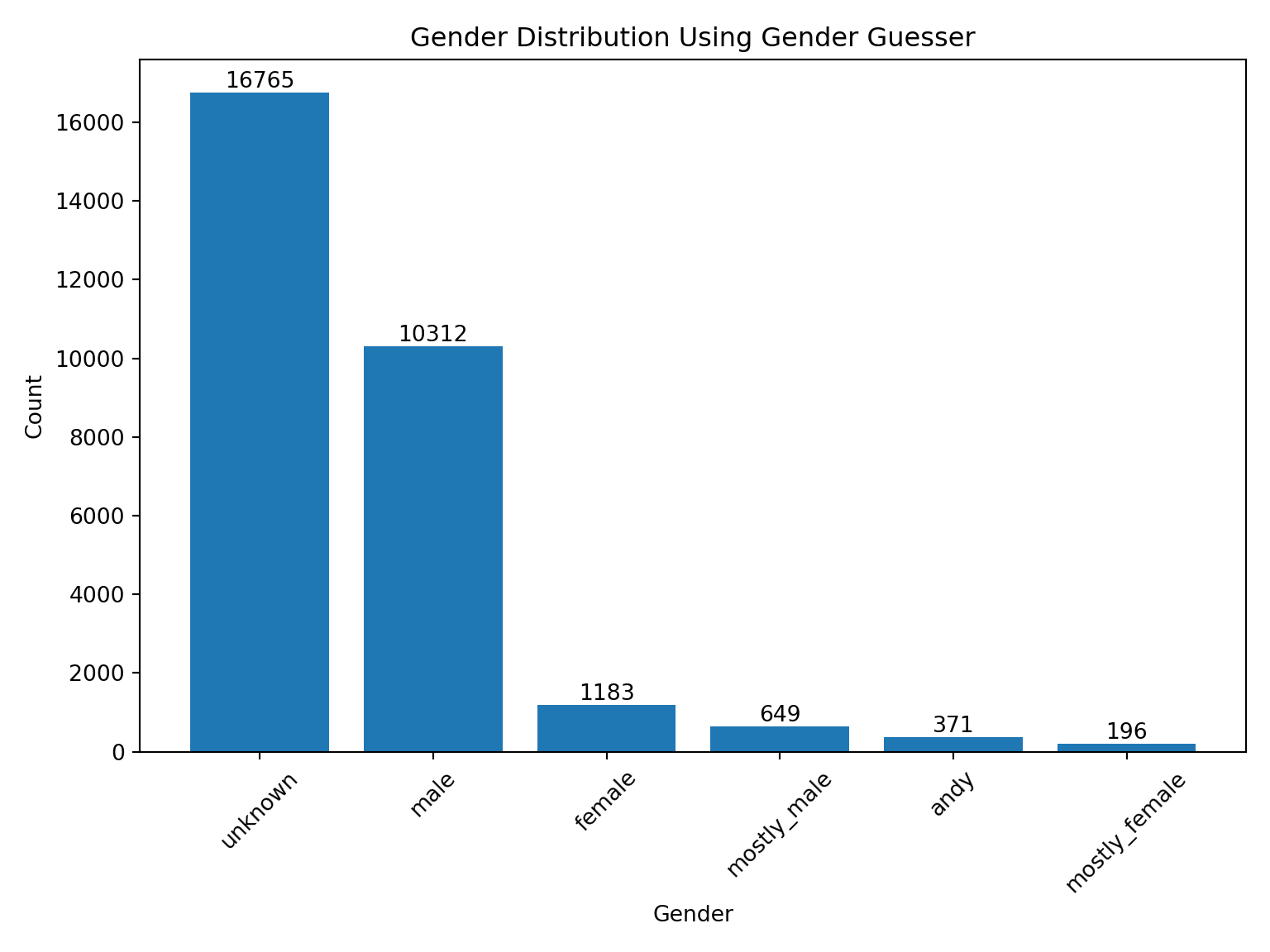
Identifying Gender Using Gender Guesser Library
This library uses the author name to predict genders. The result will be one of unknown (name not found), andy (androgynous), male, female, mostly_male, or mostly_female. The difference between andy and unknown is that the former is found to have the same probability to be male than to be female, while the later means that the name wasn’t found in the database. (Source: gender_guesser)
Code
user['assump1']=np.where(user.author_name.str.split().str.len()==2,1,0)user['namelist']=user.author_name.str.split()user['fn']=np.where(user.assump1==1,user.namelist.str[0],"NONE")unique_names=user.fn.unique()gendict={}d = gender.Detector(case_sensitive=True)for name in unique_names: g=d.get_gender(name) gendict[name]=g#Create dataframe for mergedf_gen=pd.DataFrame(list(gendict.items()),columns=['fn','genderguess'])#Merge into main file based on fnuser=user.merge(df_gen, how='left', left_on='fn', right_on='fn')import matplotlib.pyplot as plt# Assuming user.gender_from_pn.value_counts() contains the value counts datavalue_counts = user.genderguess.value_counts(dropna=False)# Create a bar chartplt.figure(figsize=(8, 6)) # Adjust the figure size as neededbars = plt.bar(value_counts.index, value_counts.values)# Add labels and titleplt.xlabel("Gender")plt.ylabel("Count")plt.title("Gender Distribution Using Gender Guesser")# Display values on top of the barsfor bar in bars: yval = bar.get_height() plt.text(bar.get_x() + bar.get_width() /2, yval, int(yval), ha='center', va='bottom')# Show the plotplt.xticks(rotation=45) # Rotate x-axis labels for better visibility if needed
plt.tight_layout() # Ensures labels are not cut offplt.show()
The dataset contains multiple entries for some individuals, with around 30% of them having more than one name therefore more than one guessed gender associated with the same login. To simplify the data, we’ll consider each unique login as representing a single individual.
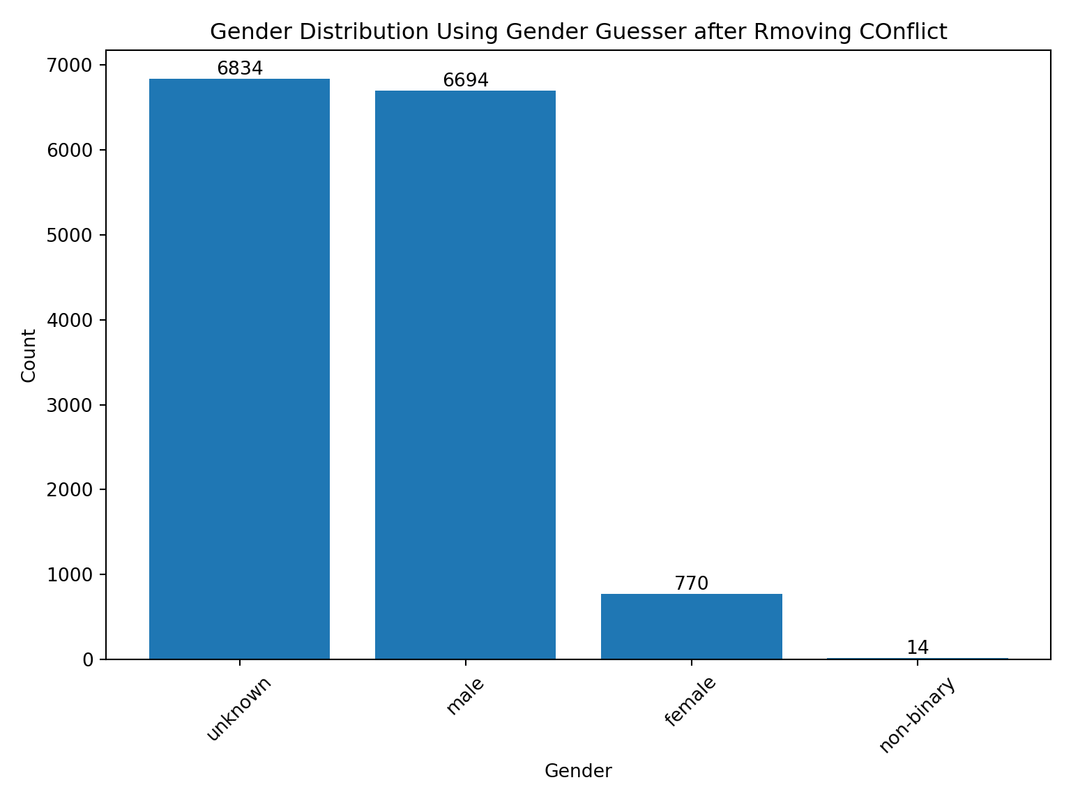
Given that individuals have more than one guessed gender, we determine the “bestguess”. If there ae signs of ambiguity, we categorize the gender as “unknown.”
List contains “female” without “andy”, “male” or “mostly male” –> female. Example: list contains female, unknown, and mostly female.
List contains “male” without “andy”, “female” or “mostly female”–> male. Example: list contains male, unknown and mostly male.
Otherwise –> unknown.
Our goal is to retain the most reliable and informative gender estimate for each person.
Code
def deconflict_genderguess(lst):if'female'in lst and'male'notin lst and'mostly male'notin lst and'andy'notin lst:return'female'if'male'in lst and'female'notin lst and'mostly female'notin lst and'andy'notin lst:return'male'else:return'unknown'user['bestguess'] = user['glist'].apply(deconflict_genderguess)user['gender'] = np.where( ((user.gender_from_pn =='male') | (user.gender_from_pn =="female") | (user.gender_from_pn =="non-binary")), user.gender_from_pn, user.bestguess)user=user.sort_values('author_user_login').groupby('author_user_login').first().reset_index()import matplotlib.pyplot as plt# Assuming user.gender_from_pn.value_counts() contains the value counts datavalue_counts = user.gender.value_counts()# Create a bar chartplt.figure(figsize=(8, 6)) # Adjust the figure size as neededbars = plt.bar(value_counts.index, value_counts.values)# Add labels and titleplt.xlabel("Gender")plt.ylabel("Count")plt.title("Gender Distribution Using Gender Guesser after Rmoving COnflict")# Display values on top of the barsfor bar in bars: yval = bar.get_height() plt.text(bar.get_x() + bar.get_width() /2, yval, int(yval), ha='center', va='bottom')# Show the plotplt.xticks(rotation=45) # Rotate x-axis labels for better visibility if needed
predicted  female  male  unknown  All
actual
female         33     3       36   72
male            4   243      144  391
All            37   246      180  463
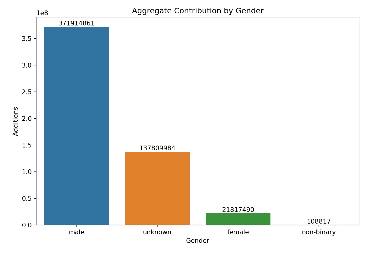
Contributions by Gender
Code
import pandas as pdimport numpy as npimport scipy.statsimport matplotlib.pyplot as pltimport seaborn as snsimport datetime as dtimport matplotlib.dates as mdates#from IPython import get_ipython#get_ipython().run_line_magic('matplotlib', 'inline')import warnings# To ignore all warnings (not recommended unless you're sure)warnings.filterwarnings("ignore")# To filter specific warning types (recommended)warnings.filterwarnings("ignore")query ='SELECT * FROM cran.commits_clean_aug4_1'# Execute the query and load the results into a DataFramecomm = pd.read_sql(query, engine)dfagg=comm.groupby(['author_login']).agg({'package':'nunique','slug': 'nunique','commit_id': 'count','additions': 'sum','deletions': 'sum','months_since_first': "first",'author_gender': 'first'}).reset_index()dfagg=dfagg.rename(columns={'package':'packages','slug': 'slugs','commit_id': 'commits','year': 'first_year','months_since_first': "tenure",'author_gender': 'author_gender'})def contribution_pivot(data, y, x):return pd.pivot_table(data, values=y, index=x, aggfunc={y:"sum"}).reset_index()tab=contribution_pivot(dfagg, 'additions', 'author_gender')tab_sorted = tab.sort_values(by='additions', ascending=False)ax=sns.barplot(x=tab_sorted.author_gender, y=tab_sorted.additions)ax.bar_label(ax.containers[0], fmt='%.0f')ax.set_ylabel('Additions')ax.set_xlabel('Gender')ax.set_title(f"Aggregate Contribution by Gender")plt.show()
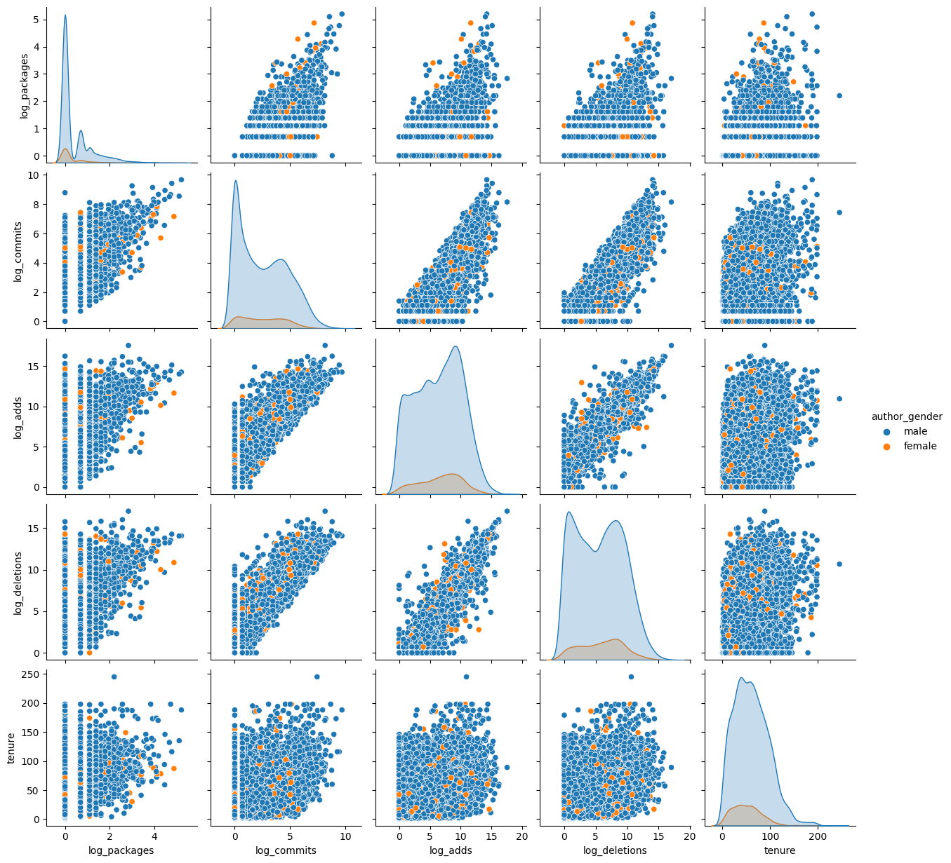
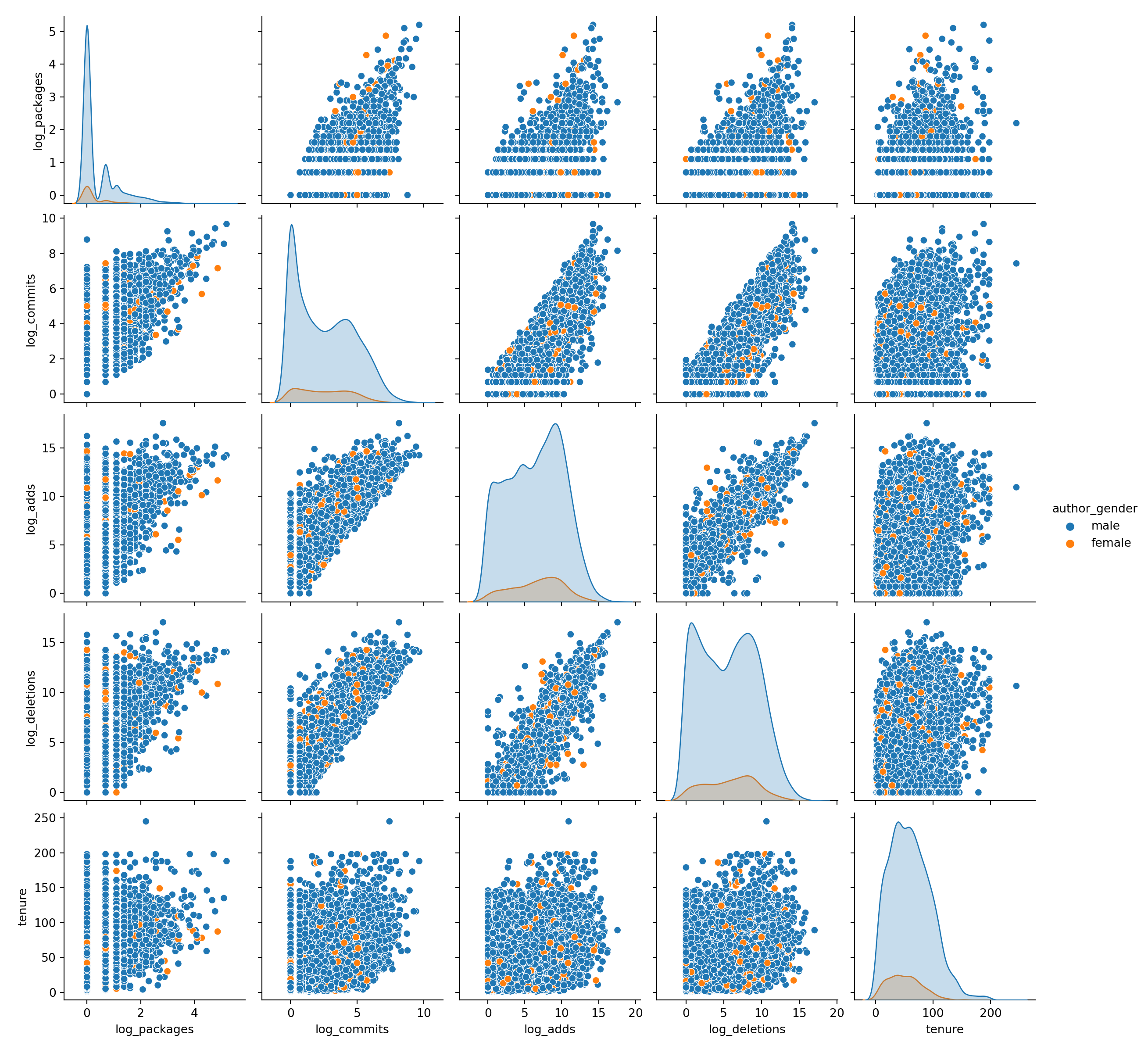
We conducted an analysis focusing on users classified as male or female, revealing bimodal log densities for both groups, suggesting the presence of two contributor categories: one with many low-volume contributors and another with a few high-volume users. Notably, additions and deletions exhibit a strong correlation of approximately 0.95, alongside correlations with commits and user tenure. This underscores the importance of normalizing contributions by tenure.
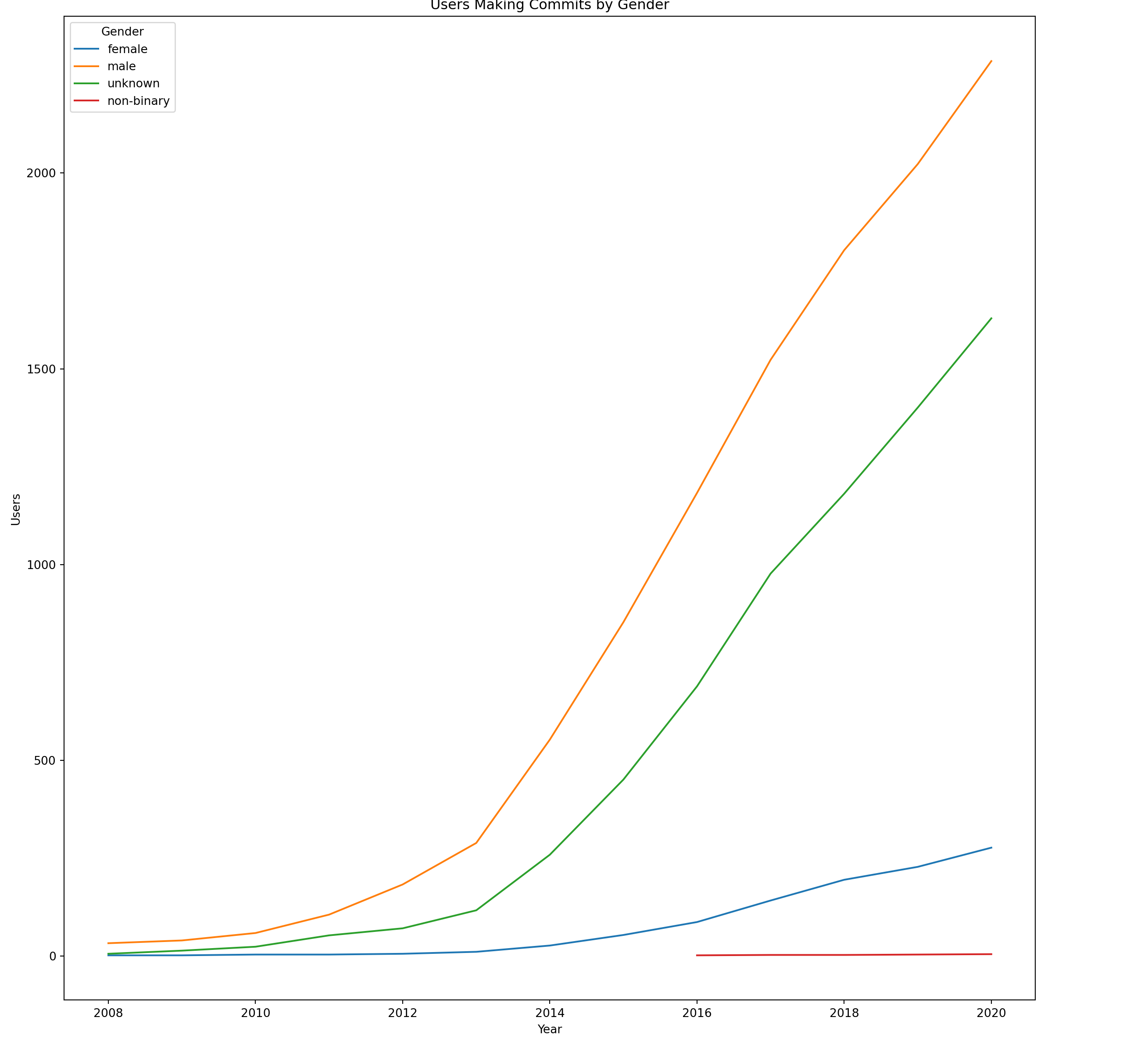
trend=comm.groupby(['author_login','year']).agg({'package':'nunique','slug': 'nunique','commit_id': 'count','additions': 'sum','deletions': 'sum','first_comm': 'first','months_since_first' : 'first','author_gender': 'first'}).reset_index()trend=trend.rename(columns={'package':'packages','slug': 'slugs','commit_id': 'commits'})max_year =2020n_years = max_year-2008trend=trend[(trend.year<=max_year)]def cagr(df,gender):return ((df[df.author_gender==gender].reset_index().iloc[n_years,3]/\ df[df.author_gender==gender].reset_index().iloc[0,3])**(1/n_years))-1#Annual count delta, 2008 to max yeardef delta(df, gender):return ((df[df.author_gender==gender].reset_index().iloc[n_years,3]-\ df[df.author_gender==gender].reset_index().iloc[0,3]))/n_yearsusers_trend=trend.groupby(["year","author_gender"]).author_login.nunique().reset_index()plot = sns.lineplot(data=users_trend, x="year", y="author_login", hue="author_gender")# Set the main title for the plotplt.title("Users Making Commits by Gender")plt.xlabel('Year')plt.ylabel('Users')# Set the legend titleplt.legend(title="Gender")# Show the plotplt.show()
Code
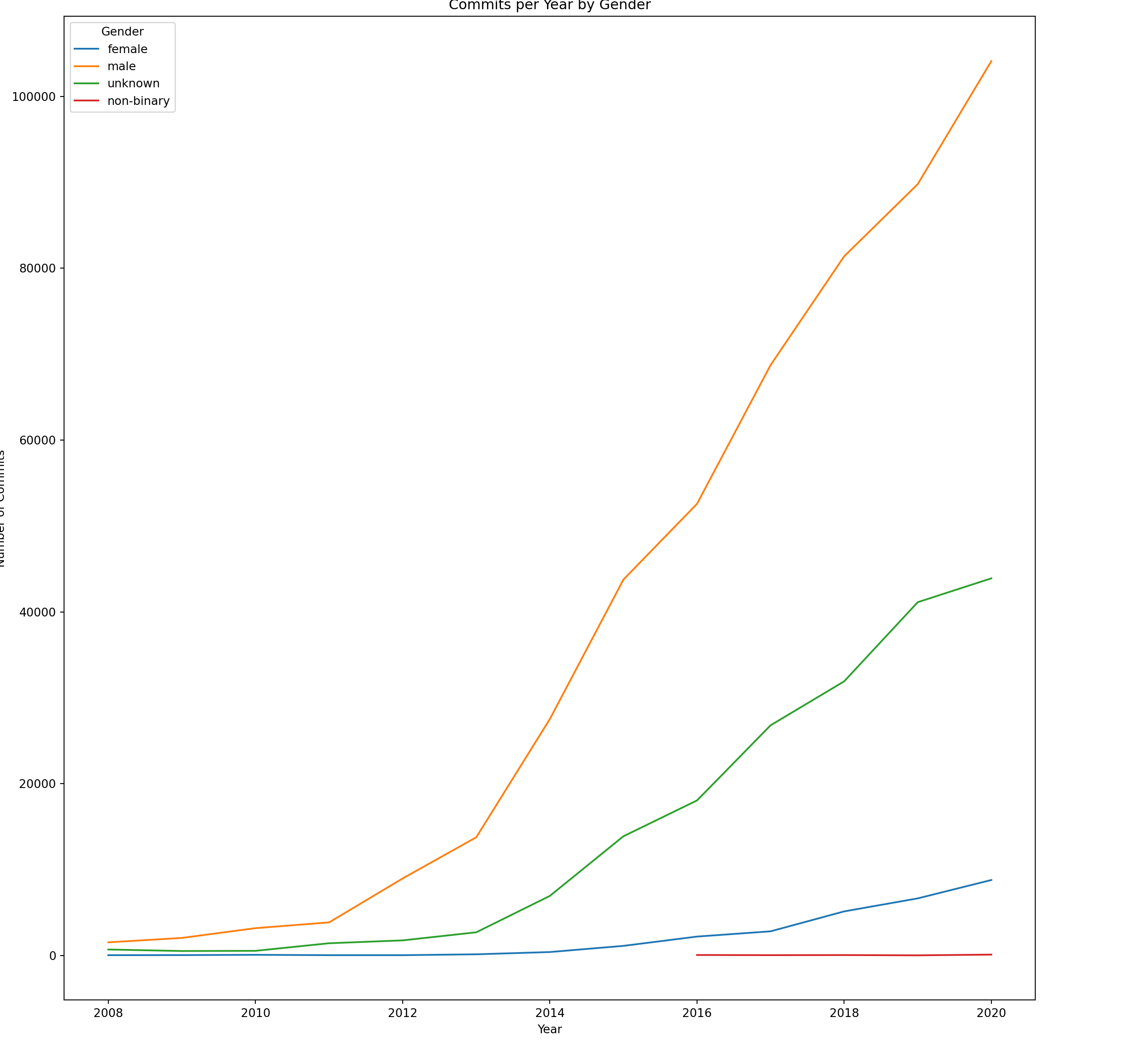
commits_trend=trend.groupby(["year","author_gender"]).commits.sum().reset_index()#commits_trendplot = sns.lineplot(data=commits_trend, x="year", y="commits", hue="author_gender").set(xlabel ='Year', ylabel ='Number of Commits', title="Commits per Year by Gender")plt.legend(title="Gender")plt.show()
Code
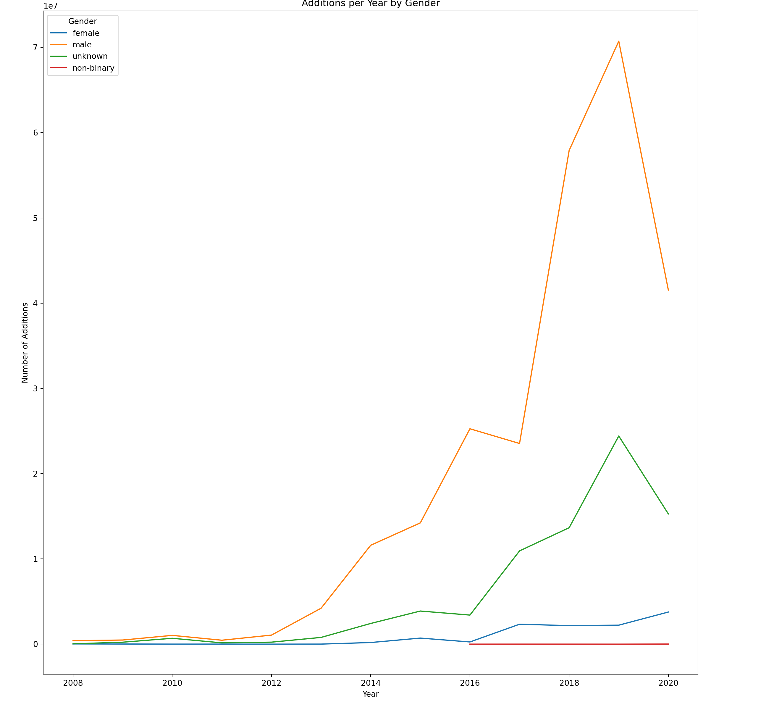
# Create plot dataadds_trend=trend.groupby(["year","author_gender"]).additions.sum().reset_index()# Line plotplot = sns.lineplot(data=adds_trend, x="year", y="additions", hue="author_gender").set(xlabel ='Year', ylabel ='Number of Additions', title="Additions per Year by Gender")plt.legend(title="Gender")plt.show()
             author_login  year packages author_gender
30219            junlingm  2023      ABM          male
8239              afmagee  2021     ACDC          male
24437              hoehna  2021     ACDC          male
3832   Jeremy-Andreoletti  2023     ACDC          male
32148            kopperud  2021     ACDC       unknown
...                   ...   ...      ...           ...
13379          cardiomoon  2018   ztable       unknown
13387          cardiomoon  2020   ztable       unknown
35668          mattocci27  2021    ztpln          male
35662          mattocci27  2018    ztpln          male
35666          mattocci27  2020    ztpln          male

[54702 rows x 4 columns]
Code
team_trend=team.groupby(['packages','year','author_gender']).agg({'author_login':'nunique'}).reset_index()team_trend_table = pd.pivot_table(team_trend, values='author_login', index=['packages', 'year'], columns=['author_gender'], aggfunc="max").reset_index().fillna(0)team_trend_table['size']=team_trend_table['female']+\ team_trend_table['male']+\ team_trend_table['non-binary']+\ team_trend_table['unknown']team_trend_table['pct_female_members'] =100*team_trend_table['female']/team_trend_table['size']team_trend_table['pct_male_members'] =100*team_trend_table['male']/team_trend_table['size']team_trend_table['pct_nb_members'] =100*team_trend_table['non-binary']/team_trend_table['size']team_trend_table['pct_unknown_members'] =100*team_trend_table['unknown']/team_trend_table['size']team_trend_table['pct_female_mfonly'] =100*team_trend_table['female']/(team_trend_table['female']+team_trend_table['male'])team_trend_dat=team_trend_table.groupby('year').agg({"pct_female_members":"mean","pct_male_members":"mean","pct_nb_members":"mean","pct_unknown_members":"mean","pct_female_mfonly":"mean"}).reset_index()sns.regplot(data=team_trend_dat, x=team_trend_dat.year.astype('int'), y='pct_female_members').\set(xlabel ='Year', ylabel ='Percentage of Female Members', title='Average %Female Contributors per Package, by Year\nDenominator Includes All Gender Categories\nMean with 95% CI');
Source Code
---title: "R Gender Analysis"editor: markdown: wrap: 72format: html: code-fold: true code-tools: true df-print: paged---## Identifying Gender Using PronounsGitHub data contains pronouns for each user, we analyse this pronouncolumn and look for unique, blank and null values```{r, include=FALSE}library(reticulate)reticulate::use_condaenv("C:/Users/rahul/anaconda3/envs/snowflakes")``````{python}#| echo: falseimport pandas as pdimport numpy as npimport gender_guesser.detector as genderfrom sqlalchemy import create_engineimport pymysqlfrom sqlalchemy import texthostname="oss-1.cij9gk1eehyr.us-east-1.rds.amazonaws.com"dbname="cran"uname="jdpinto"pwd="DSPG2023"# Create SQLAlchemy engine to connect to MySQL Databaseengine = create_engine("mysql+pymysql://{user}:{pw}@{host}/{db}".format(host=hostname, db=dbname, user=uname, pw=pwd))query ='SELECT * FROM cran.cran_users'# Execute the query and load the results into a DataFrameuser = pd.read_sql(query, engine)def check_var(df,var): unique=df[var].nunique() blanks = df[df[var]==""].shape[0] nans = df[var].isna().sum()print("Unique values: ", unique, "\nBlanks: ", blanks, "\nNaNs: ", nans)print('For pronouns present in GitHub data: ')check_var(user, 'author_user_pronouns')```While analyzing the pronoun data we found these pronouns entered by theusers:```{python}invalid_cases=['Zurich, Switzerland','Chicago, IL, USA','Denver, CO','Wellington, New Zealand','Omaha, NE','Durham, UK','Barcelona','Flagstaff, AZ','Bamberg, Germany','Ghent, Belgium','Sydney, AUS','Melbourne, Australia','Brazil','Nashville, TN','Munich','Wellington, New Zealand','USA','Data welder 👨\u200d🏭 and Research Scientist']# user[user.author_user_login.isin(invalid_cases)][['author_user_login','author_name','author_email','author_user_location','author_user_pronouns']]user=user[~user.author_user_login.isin(invalid_cases)]pronoun_data = user['author_user_pronouns'].value_counts().to_dict()pronoun_data```Using this data we divide users four categories: male, female,non-binary and unknown.```{python}gender_map = {np.nan: "Missing","" : "Missing",'he/him': "male",'she/her': "female",'they/them': "non-binary" ,'any': "Missing",'she/they': "female",'he/they': "male",'he/him/point': "male",'he/they/she': "non-binary",'(any pronouns)': "Missing",'they/he': "male",'he/him or whatever': "male",'he/him/any': "male",'Walmart Bag': "Missing",'Ojisan': "Missing",'🐈': "Missing"}user['gender_from_pn'] = user['author_user_pronouns'].map(gender_map)import matplotlib.pyplot as plt# Assuming user.gender_from_pn.value_counts() contains the value counts datavalue_counts = user.gender_from_pn.value_counts()# Create a bar chartplt.figure(figsize=(8, 6)) # Adjust the figure size as neededbars = plt.bar(value_counts.index, value_counts.values)# Add labels and titleplt.xlabel("Gender")plt.ylabel("Count")plt.title("Gender Distribution using Pronouns")# Display values on top of the barsfor bar in bars: yval = bar.get_height() plt.text(bar.get_x() + bar.get_width() /2, yval, int(yval), ha='center', va='bottom')# Show the plotplt.xticks(rotation=45) # Rotate x-axis labels for better visibility if neededplt.tight_layout() # Ensures labels are not cut offplt.show()```## Identifying Gender Using Gender Guesser LibraryThis library uses the author name to predict genders. The result will beone of unknown (name not found), andy (androgynous), male, female,mostly_male, or mostly_female. The difference between andy and unknownis that the former is found to have the same probability to be male thanto be female, while the later means that the name wasn't found in thedatabase. (Source:[gender_guesser](https://pypi.org/project/gender-guesser/))```{python}user['assump1']=np.where(user.author_name.str.split().str.len()==2,1,0)user['namelist']=user.author_name.str.split()user['fn']=np.where(user.assump1==1,user.namelist.str[0],"NONE")unique_names=user.fn.unique()gendict={}d = gender.Detector(case_sensitive=True)for name in unique_names: g=d.get_gender(name) gendict[name]=g#Create dataframe for mergedf_gen=pd.DataFrame(list(gendict.items()),columns=['fn','genderguess'])#Merge into main file based on fnuser=user.merge(df_gen, how='left', left_on='fn', right_on='fn')import matplotlib.pyplot as plt# Assuming user.gender_from_pn.value_counts() contains the value counts datavalue_counts = user.genderguess.value_counts(dropna=False)# Create a bar chartplt.figure(figsize=(8, 6)) # Adjust the figure size as neededbars = plt.bar(value_counts.index, value_counts.values)# Add labels and titleplt.xlabel("Gender")plt.ylabel("Count")plt.title("Gender Distribution Using Gender Guesser")# Display values on top of the barsfor bar in bars: yval = bar.get_height() plt.text(bar.get_x() + bar.get_width() /2, yval, int(yval), ha='center', va='bottom')# Show the plotplt.xticks(rotation=45) # Rotate x-axis labels for better visibility if neededplt.tight_layout() # Ensures labels are not cut offplt.show()```The dataset contains multiple entries for some individuals, with around30% of them having more than one name therefore more than one guessedgender associated with the same login. To simplify the data, we'llconsider each unique login as representing a single individual.```{python}user['china'] = user.author_user_location.str.lower().str.find("china")user['india'] = user.author_user_location.str.lower().str.find("india")user['japan'] = user.author_user_location.str.lower().str.find("japan")user['korea'] = user.author_user_location.str.lower().str.find("korea")gender_name_manual={'Andrea':"unknown","Drea":"female","Jin": "unknown","June": "unknown","Jun": "unknown","Lele": "unknown","Anush": "male"}user['manual_gender'] = user['fn'].map(gender_name_manual)user['nemail'] = user.groupby('author_user_login')['author_email'].transform('nunique')user['n_name'] = user.groupby('author_user_login')['author_name'].transform('nunique')user['n_pronoun'] = user.groupby('author_user_login')['author_user_pronouns'].transform('nunique')user['n_gen_from_pn'] = user.groupby('author_user_login')['gender_from_pn'].transform('nunique')user['n_genderguess'] = user.groupby('author_user_login')['genderguess'].transform('nunique')#How many unique logins does each email haveuser['n_login_per_email'] = user.groupby('author_email')['author_user_login'].transform('nunique')def make_list_vars(df1,group_var,target_var): df2=pd.DataFrame(user.groupby(group_var)[target_var].apply(lambda x: x.tolist())).reset_index() df2=df2.rename({target_var:str(target_var)[0] +"list"}, axis=1)return df1.merge(df2, how="left", left_on="author_user_login", right_on="author_user_login")user=make_list_vars(user, 'author_user_login', 'genderguess')user[user.author_user_login=="Mamba413"][['author_user_login','author_name','genderguess','n_genderguess','glist']]```Given that individuals have more than one guessed gender, we determinethe "bestguess". If there ae signs of ambiguity, we categorize thegender as "unknown."- List contains "female" without "andy", "male" or "mostly male" --\> female. Example: list contains female, unknown, and mostly female.- List contains "male" without "andy", "female" or "mostly female"--\> male. Example: list contains male, unknown and mostly male.- Otherwise --\> unknown.Our goal is to retain the most reliable and informative gender estimatefor each person.```{python}def deconflict_genderguess(lst):if'female'in lst and'male'notin lst and'mostly male'notin lst and'andy'notin lst:return'female'if'male'in lst and'female'notin lst and'mostly female'notin lst and'andy'notin lst:return'male'else:return'unknown'user['bestguess'] = user['glist'].apply(deconflict_genderguess)user['gender'] = np.where( ((user.gender_from_pn =='male') | (user.gender_from_pn =="female") | (user.gender_from_pn =="non-binary")), user.gender_from_pn, user.bestguess)user=user.sort_values('author_user_login').groupby('author_user_login').first().reset_index()import matplotlib.pyplot as plt# Assuming user.gender_from_pn.value_counts() contains the value counts datavalue_counts = user.gender.value_counts()# Create a bar chartplt.figure(figsize=(8, 6)) # Adjust the figure size as neededbars = plt.bar(value_counts.index, value_counts.values)# Add labels and titleplt.xlabel("Gender")plt.ylabel("Count")plt.title("Gender Distribution Using Gender Guesser after Rmoving COnflict")# Display values on top of the barsfor bar in bars: yval = bar.get_height() plt.text(bar.get_x() + bar.get_width() /2, yval, int(yval), ha='center', va='bottom')# Show the plotplt.xticks(rotation=45) # Rotate x-axis labels for better visibility if neededplt.tight_layout() # Ensures labels are not cut offplt.show()```## Confusion Matrix: Self-Reported Pronouns vs. Guessed Gender```{python}g_map={'unknown':'unknown','female':'female','male':'male','non-binary':'other','Missing':'unknown'}user['predicted'] = user['bestguess'].map(g_map)user['actual'] = user['gender_from_pn'].map(g_map)cmdata=user[(user.actual!="other") & (user.actual!="unknown")][['author_user_login','predicted','actual']]pd.crosstab(cmdata.actual,cmdata.predicted, margins=True)```## Contributions by Gender```{python}import pandas as pdimport numpy as npimport scipy.statsimport matplotlib.pyplot as pltimport seaborn as snsimport datetime as dtimport matplotlib.dates as mdates#from IPython import get_ipython#get_ipython().run_line_magic('matplotlib', 'inline')import warnings# To ignore all warnings (not recommended unless you're sure)warnings.filterwarnings("ignore")# To filter specific warning types (recommended)warnings.filterwarnings("ignore")query ='SELECT * FROM cran.commits_clean_aug4_1'# Execute the query and load the results into a DataFramecomm = pd.read_sql(query, engine)dfagg=comm.groupby(['author_login']).agg({'package':'nunique','slug': 'nunique','commit_id': 'count','additions': 'sum','deletions': 'sum','months_since_first': "first",'author_gender': 'first'}).reset_index()dfagg=dfagg.rename(columns={'package':'packages','slug': 'slugs','commit_id': 'commits','year': 'first_year','months_since_first': "tenure",'author_gender': 'author_gender'})def contribution_pivot(data, y, x):return pd.pivot_table(data, values=y, index=x, aggfunc={y:"sum"}).reset_index()tab=contribution_pivot(dfagg, 'additions', 'author_gender')tab_sorted = tab.sort_values(by='additions', ascending=False)ax=sns.barplot(x=tab_sorted.author_gender, y=tab_sorted.additions)ax.bar_label(ax.containers[0], fmt='%.0f')ax.set_ylabel('Additions')ax.set_xlabel('Gender')ax.set_title(f"Aggregate Contribution by Gender")plt.show()dat=dfagg#dat=dfagg[(dfagg.author_gender=="male")|(dfagg.author_gender=="female")]table=pd.pivot_table(dat, values=['author_login','deletions','commits','additions','packages'], index=['author_gender'], aggfunc={'author_login':"nunique",'commits' : "sum",'additions': "sum",'deletions': "sum"})table['percent_gender'] =round((table['author_login']/table['author_login'].sum())*100,2)table['percent_adds'] =round((table['additions']/table['additions'].sum())*100,2)table['percent_commits'] =round((table['commits']/table['commits'].sum())*100,2)table['percent_deletions'] =round((table['deletions']/table['deletions'].sum())*100,2)table=table.rename(columns={"author_login": 'gender_count'})table[['percent_gender','percent_adds','percent_commits','percent_deletions']]```## Correlation:We conducted an analysis focusing on users classified as male or female,revealing bimodal log densities for both groups, suggesting the presenceof two contributor categories: one with many low-volume contributors andanother with a few high-volume users. Notably, additions and deletionsexhibit a strong correlation of approximately 0.95, alongsidecorrelations with commits and user tenure. This underscores theimportance of normalizing contributions by tenure.```{python}dfagg['log_packages']=np.log(dfagg['packages'])dfagg['log_commits']=np.log(dfagg['commits'])dfagg['log_adds']=np.log(dfagg['additions'])dfagg['log_deletions']=np.log(dfagg['deletions'])mfonly=dfagg[(dfagg.author_gender=="male")| (dfagg.author_gender=="female")]mfonly=mfonly[['log_packages','log_commits','log_adds', 'log_deletions','tenure','author_gender']]sns.pairplot(mfonly, hue="author_gender")plt.show()```## Gender Differences in OSS Development Over Time```{python}trend=comm.groupby(['author_login','year']).agg({'package':'nunique','slug': 'nunique','commit_id': 'count','additions': 'sum','deletions': 'sum','first_comm': 'first','months_since_first' : 'first','author_gender': 'first'}).reset_index()trend=trend.rename(columns={'package':'packages','slug': 'slugs','commit_id': 'commits'})max_year =2020n_years = max_year-2008trend=trend[(trend.year<=max_year)]def cagr(df,gender):return ((df[df.author_gender==gender].reset_index().iloc[n_years,3]/\ df[df.author_gender==gender].reset_index().iloc[0,3])**(1/n_years))-1#Annual count delta, 2008 to max yeardef delta(df, gender):return ((df[df.author_gender==gender].reset_index().iloc[n_years,3]-\ df[df.author_gender==gender].reset_index().iloc[0,3]))/n_yearsusers_trend=trend.groupby(["year","author_gender"]).author_login.nunique().reset_index()plot = sns.lineplot(data=users_trend, x="year", y="author_login", hue="author_gender")# Set the main title for the plotplt.title("Users Making Commits by Gender")plt.xlabel('Year')plt.ylabel('Users')# Set the legend titleplt.legend(title="Gender")# Show the plotplt.show()commits_trend=trend.groupby(["year","author_gender"]).commits.sum().reset_index()#commits_trendplot = sns.lineplot(data=commits_trend, x="year", y="commits", hue="author_gender").set(xlabel ='Year', ylabel ='Number of Commits', title="Commits per Year by Gender")plt.legend(title="Gender")plt.show()# Create plot dataadds_trend=trend.groupby(["year","author_gender"]).additions.sum().reset_index()# Line plotplot = sns.lineplot(data=adds_trend, x="year", y="additions", hue="author_gender").set(xlabel ='Year', ylabel ='Number of Additions', title="Additions per Year by Gender")plt.legend(title="Gender")plt.show()team=comm.groupby(['author_login','year','package']).agg({'author_gender': 'first'}).reset_index()team=team.rename(columns={'package':'packages'})team.sort_values('packages')team_trend=team.groupby(['packages','year','author_gender']).agg({'author_login':'nunique'}).reset_index()team_trend_table = pd.pivot_table(team_trend, values='author_login', index=['packages', 'year'], columns=['author_gender'], aggfunc="max").reset_index().fillna(0)team_trend_table['size']=team_trend_table['female']+\ team_trend_table['male']+\ team_trend_table['non-binary']+\ team_trend_table['unknown']team_trend_table['pct_female_members'] =100*team_trend_table['female']/team_trend_table['size']team_trend_table['pct_male_members'] =100*team_trend_table['male']/team_trend_table['size']team_trend_table['pct_nb_members'] =100*team_trend_table['non-binary']/team_trend_table['size']team_trend_table['pct_unknown_members'] =100*team_trend_table['unknown']/team_trend_table['size']team_trend_table['pct_female_mfonly'] =100*team_trend_table['female']/(team_trend_table['female']+team_trend_table['male'])team_trend_dat=team_trend_table.groupby('year').agg({"pct_female_members":"mean","pct_male_members":"mean","pct_nb_members":"mean","pct_unknown_members":"mean","pct_female_mfonly":"mean"}).reset_index()sns.regplot(data=team_trend_dat, x=team_trend_dat.year.astype('int'), y='pct_female_members').\set(xlabel ='Year', ylabel ='Percentage of Female Members', title='Average %Female Contributors per Package, by Year\nDenominator Includes All Gender Categories\nMean with 95% CI');```